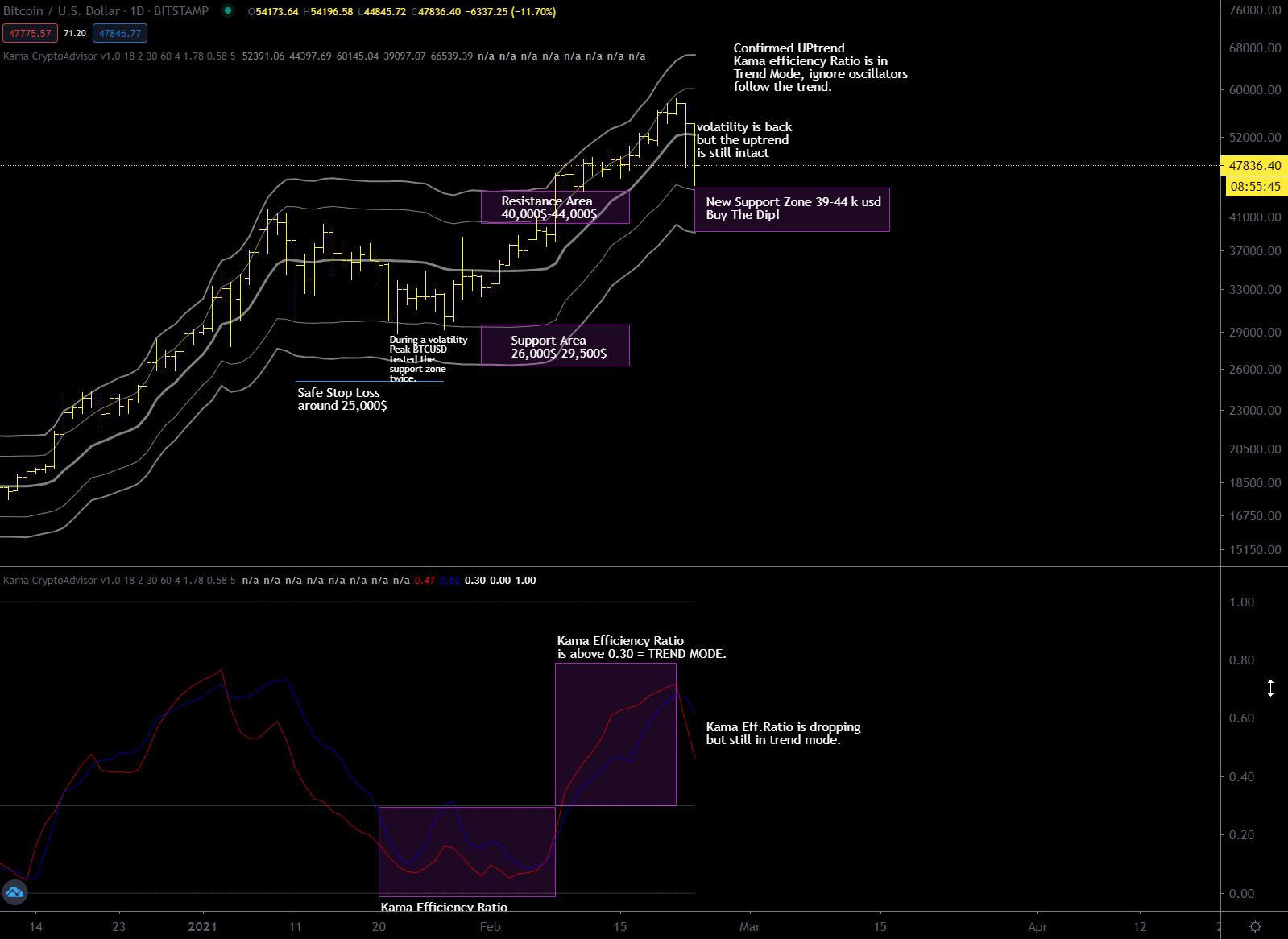
The volatility is back, to be honest I had suspected two days ago that Bitcoin was running out of fuel, even some profit taking evident on the hourly chart had let me think so and then yesterday that volatility peak was the confirmation. Despite this, at a careful and lucid analysis, the situation on the daily chart has not changed, we are still in trend mode and it is not guaranteed that Bitcoin will go sideways in the next days. In any case, pay particular attention to the support zone between 39 and 44 thousand dollars, it is very important to stay above 39 thousand dollars in order not to compromise the ongoing bullish trend.
BTCUSD Daily Chart – Kama average and deviation bands | Kama efficiency ratio
The most keen observers will have noticed that after a prolonged bullish trend, the kama efficiency ratio had reached 0.71, which is beginning to be an important value. Personally I see the correction of these two days as absolutely normal and also necessary in order to continue. I would also add that this market did not go down because of Janet Yellen’s statements, news are always a consequence of market forces and never the cause. I explained in the past, for those who have been following me for some time on the blog, that when a bearish phase starts, the negative news will be amplified and the positive ones ignored, vice versa when a bullish phase starts, the negative news will be ignored and the positive ones will be amplified, but it is never the news in itself that moves the market.
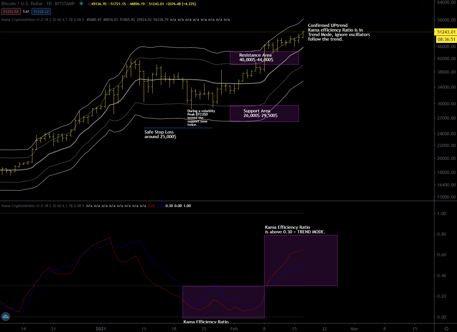
I waited a while before updating you about the short term situation because i wanted to see if the trend confirmed by the Kama efficiency rate was good and not a false signal.
BTCUSD – Daily Chart View
As I have said many times in the past, when the Kama average is flat there are very good resistance and support zones that define the useful space in which an asset, in this case bitcoin, moves. Outside of these resistance zones a trend reversal is confirmed (if we break the support zone) or the continuation of the bullish trend (if we break the resistance zone). What has happened is that bitcoin has broken the resistance zone positioned at 40-44 thousand dollars thus confirming the bullish trend. On the weekly chart the trend is strong and price remains consistently above the weekly Kama average. Kama efficiency ratio is now in “Trend Mode” on all the main timeframes: Daily, Weekly, Monthly; therefore my outlook is strongly bullish.
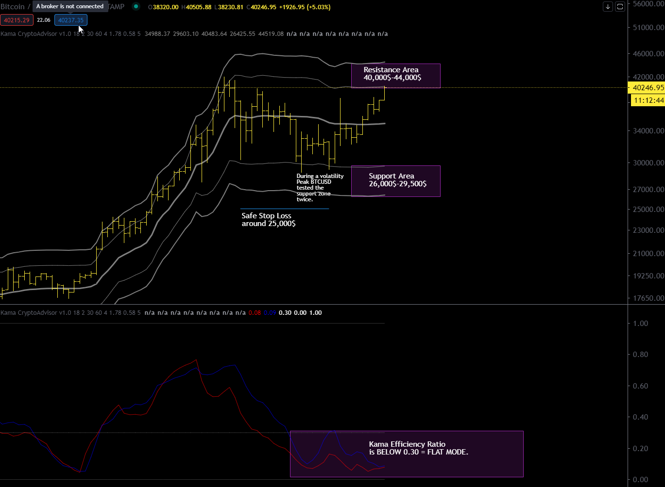
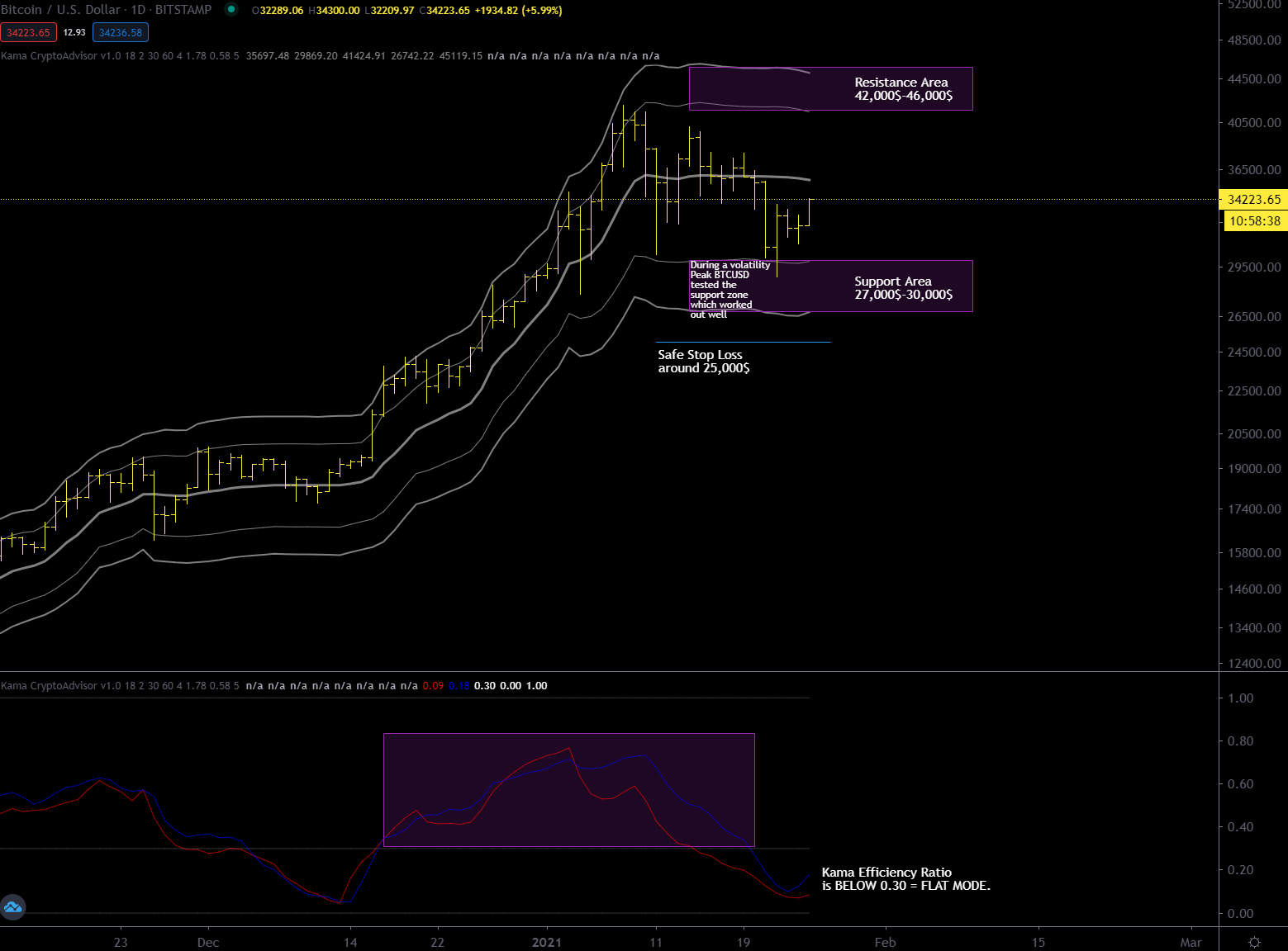
The situation has not changed much since the last update, BTCUSD retested the support zone a second time and reacted to the upside. Now we are entering the resistance zone and the kama efficiency ratio is still below 0.30, flat market. I would say that I’ll expect some form of resistance between 40 and 44k from sellers in general. A decisive break above $44k would confirm the continuation of the ongoing bullish trend on the monthly chart.
BTCUSD Daily Chart – Kama average and bands + Kama Efficiency Ratio
A particular attention deserves the situation on the weekly chart, where instead of going down BTCUSD remained flat for 4 weeks, I would interpret this behavior as a signal of strength. Honestly, looking at the weekly chart, I already see 53-54 thousand dollars as a target for the coming weeks.
OFFTOPIC: A nice example of how to spot a top with Kama Efficiency Ratio
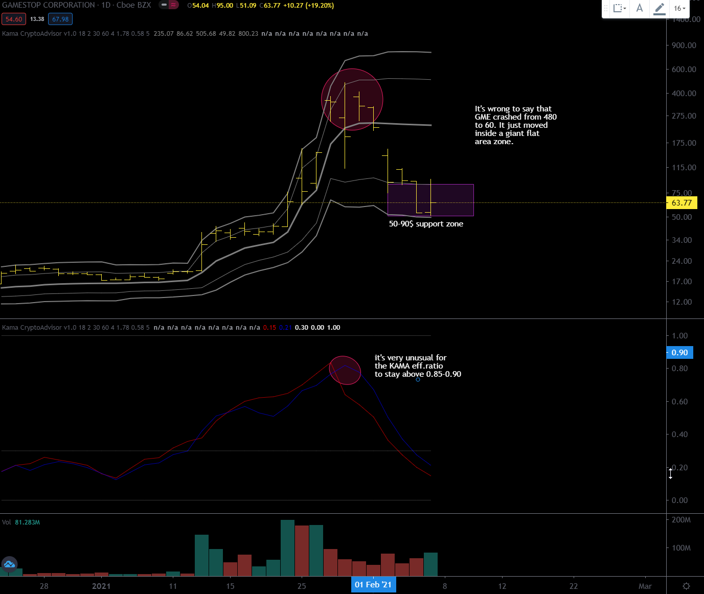
GME Daily Chart – Kama and Kama ER
I wanted to include this example because I think it is very good to understand the potential of the Kama average togheter with deviation bands and its efficiency rate (ER). Last 28 January after a very volatile day and given the reading of over 0.80 of the kama ER I understood that something was wrong and that the top could have been done. This was confirmed in the following days. A violent downward movement immediately brings the average kama in a stalemate position that allows us to have reliable deviation bandssupport/resistance zone. I expected a correction down to 60 usd, which then happened. It is also not correct to say that the price collapsed from $480 to $60, it just moved within a very wide flat zone. Now the GME price might even go back up to the Kama average.
Since the last daily update bitcoin has gone into “flat mode” (kama efficiency ratio below 0.30), in this mode you can expect the oscillators to work fairly well so that the widespread stochastic oscillator gave you a nice buy signal a few days ago. I believe that today or tomorrow at the latest bitcoin is going to recover the Kama average at $35,900. It remains to be seen in which direction the kama efficiency ratio will confirm the next trend on the daily chart considering that the situation on the weekly remains a bit unfavorable to the bullish while the monthly one is not, as I said in the previous long term update of January 19.
BTCUSD Daily Chart – Kama and Kama efficiency ratio, 18 periods.
The Efficiency Ratio (from now on ER) was presented by Perry Kaufman in his 1995 book “Smarter Trading” and it is calculated by dividing the price change over a fixed number of bars by the sum of the price movements that occurred to achieve that change. The resulting ratio ranges between 0 and 1 with higher values representing a more trending market. The idea here is to measure the value of the ER during an important Bitcoin Top to see if there is a strong coherence between different timeframes.
Date
Daily ER
Weekly ER
Monthly ER
Average of 3
November 30, 2013
0.70
0.79
0.64
0.71
December 18, 2017
0.66
0.74
0.88
0.76
January 8 , 2021
0.62
0.77
0.44
0.61
Multi TimeFrame Kama Efficiency Ratio at Bitcoin Historical Tops
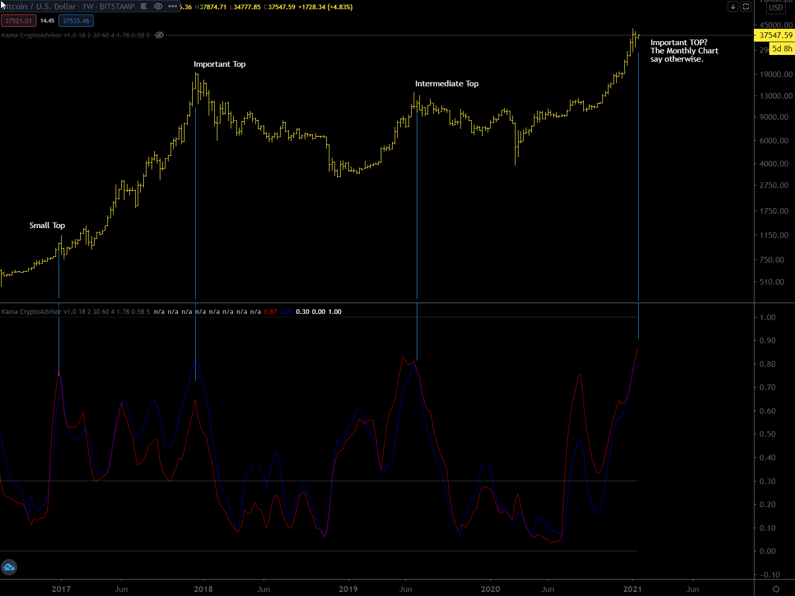
The high of last January 8 does not seem to have a situation on the various timeframes similar to that one of two important Bitcoin top (2013 and 2017), in particular the situation on the monthly timeframe is inconsistent. On the weekly timeframe instead ER is quite high but I think that in the end the monthly timeframe will prevail. It is always difficult to understand which timeframe dominates over the others but personally I prefer to give precedence to the highest timeframe, in this case the monthly where there is room to rise. I attach below the weekly chart so you can better visualize the ER situation
Weekly Chart BTCUSD with Kama Efficieny Ratio
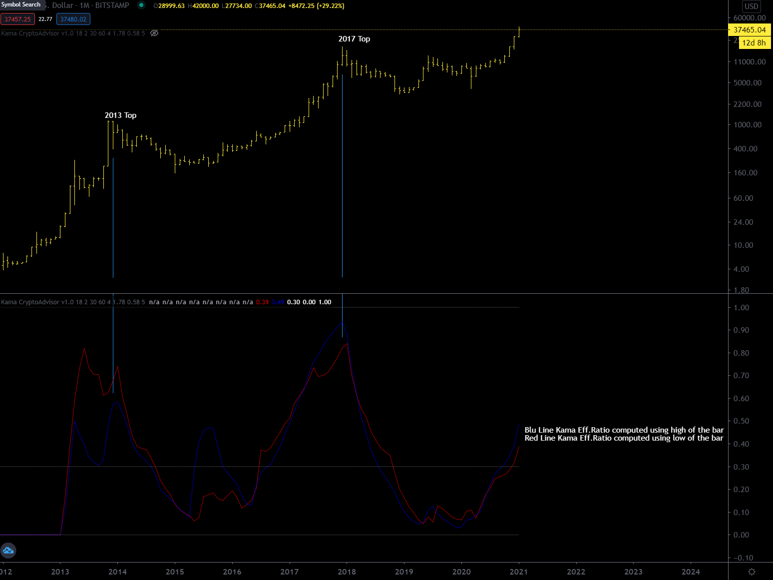
And here the monthly chart where you can clearly see there is room for a prolonged trend.
BTCUSD Monthly Chart with 18 periods Kama Efficiency Ratio
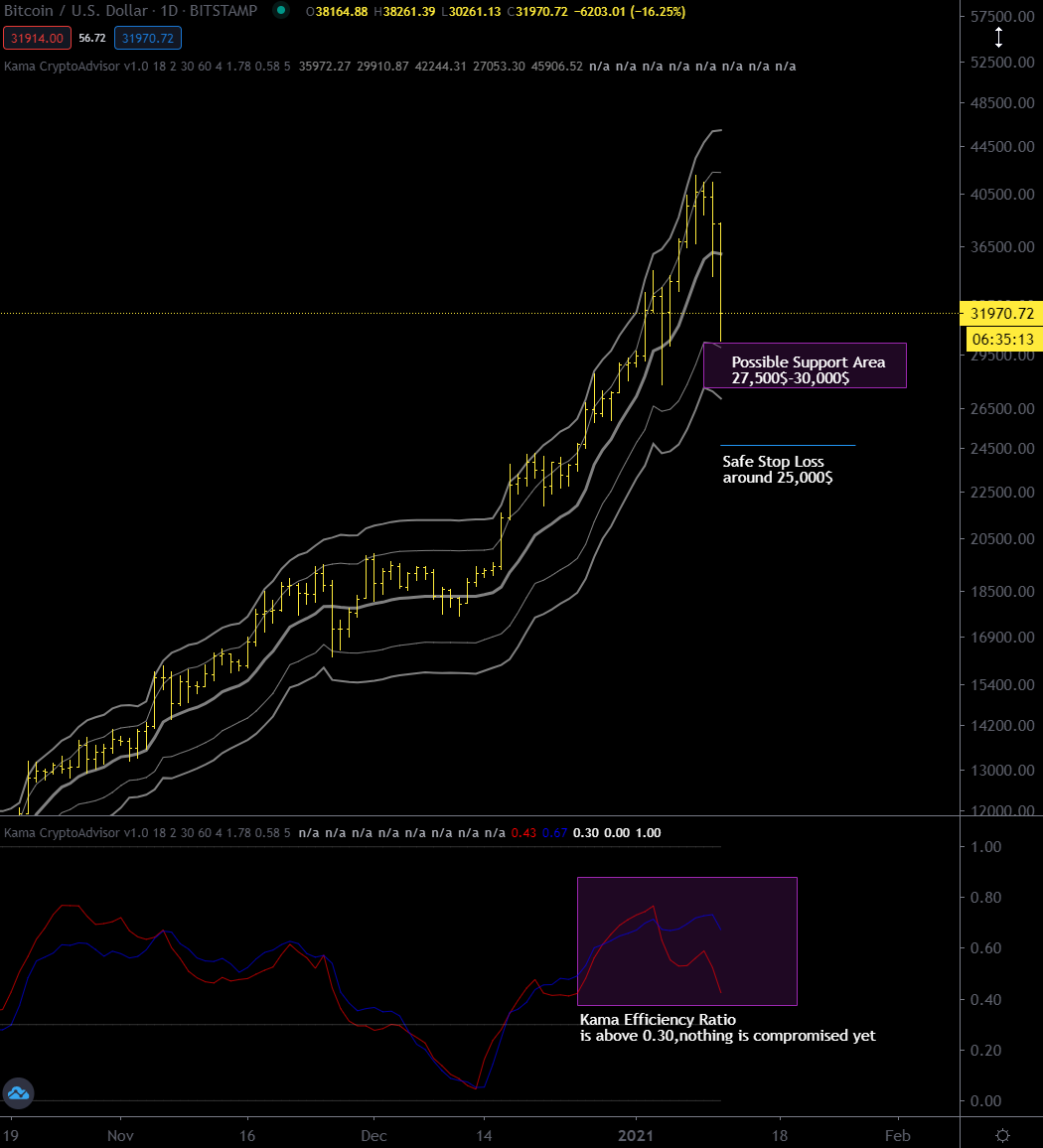
I always tell you guys that it is very important to evaluate the relationship between trend strength and volatility, it makes us understand if the market is in “trend mode” or “flat mode”, at the moment we are at the limits, the market has reacted from the support shown in the last update but it is not enough. In order to stay in “trend mode” it is now necessary to make a higher top than the previous one, perhaps around $46,000; any top lower then this would imply that BTCUSD is slowing down and going FLAT.
BTCUSD Daily Chart – Kama deviation bands and efficiency ratio on lower pane
When a security or an asset is in “trend mode” it is strategically optimal to keep the position in the direction of the trend without trying to go against by opening a short positions inside the deviation bands resistance area. If you really want to go short, enhance the efficiency of your initial stop-loss by pairing it with a trailing stop loss.
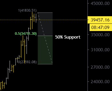
I didn’t expect such an intense drop, as a general rule when volatility increases you have to go up with the timeframe used, the 4 hour chart is not enough anymore. On the daily chart a correction below $30,000 would mean that an intermediary top has been made at $42,000 and that a more or less prolonged sideways movement awaits us before seeing new highs. I am including below an updated daily chart.
After a strong rise from $27,000 to $42,000 I think it is time for a break, in these situations sometimes the simplest approach is the valid one. The most obvious support is the 50% of the range at around 34,800$.
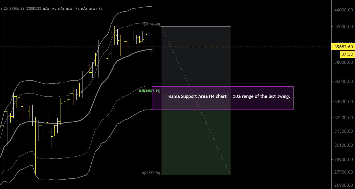
The closest dynamic support are the deviation bands of the kama average on the 4 hour timeframe.
I’m not saying that BTCUSD will go there, it could be an opportunity to buy if this scenario materializes. Don’t forget that when the market is fast you can lower the timeframe to find better support areas, as you can see in the above chart KAMA deviation bands worked well during the sell-off down to 27,000$ last January 4. Under these circumstances the daily chart is too slow to adapt.
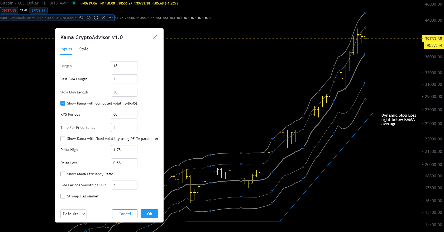
You often ask me when to enter a trend already started, usually it is never too late to buy the important thing is to place a stop that is beyond the deviation bands that I use, to stay safe from volatility.
Let’s see an example on the daily chart.
BTCUSD Daily Chart with kama average and an ideal dynamic stoploss – KAMA parameters that i use are included.
You can buy at any moment a well established trend but keep in mind that the right stoploss to use is wide, not tight because Bitcoin volatility is high. If you don’t like KAMA average and the way i compute bands you can give a try to Keltner Channels. Personally i prefer the approach of Mr.Kaufman but the choice is yours.
Every year i post an outlook using entropic methods explained in the technical section of this blog. Here you can find the 2015, 2016,2017,2018 , 2019 and 2020, forecast update, where you can find more information about this approach.
Updated values for bitcoin (in brackets values of last year) using daily data since August 2010 (average data of 4 important exchanges when possible).
BTC/USD
Growth Factor G
1.00104 (1.00087)
Shannon Probability P
0.5232 (0.5219)
Root mean square RMS (see this as volatility)
0.055 (0.056 )
Bitcoin’s entropic values versus the Usd improved during 2020, the Growth Factor (G) grow to 1.00104% compounded daily or 146% yearly, higher then 1y ago. The optimal fraction of your total wealth to invest in bitcoin rised to 4.6% (~0.5232*2=1.046 – 1 = 0.046 or 4.6% roundable to 5%). Volatility continues to drop year after year and that’s normal as bitcoin gets bigger and bigger so less prone to volatility. These values are still much better then conventional markets except the Shannon Probability that still match the US Stock Markets (around 0.522); it means that out of 100 days an asset goes up 52 days and down for 48 days, on average.
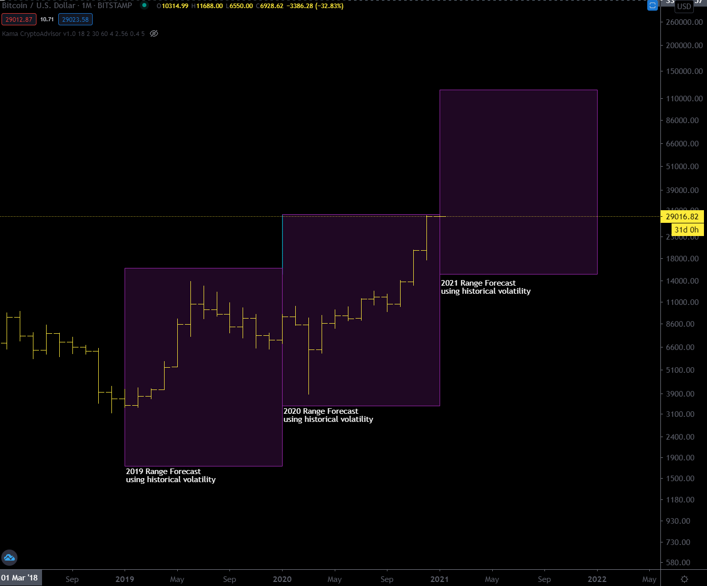
2021 Price forecast
Full Historical Volatility
Half Historical Volatility
Forecast using only G*
~42,400$
~42,400$
Upper bound adding volatility
~121,000$
~71,850$
Lower bound subtracting volatility
~14,750$
~25,000$
*42400 is obtained with 1st January as a starting price (around 28985$) times (1.00104^365)=~1.463 | 28985*1.463=~42400, just change 365 with the number of days you prefer for a different forecast.
What happened in 2020?
A year ago, I forecasted a maximum top of $29380 almost reached the last day of the year. This market has made a low in March that I like to call a “selling climax bottom” when the bearish momentum is exhausted during a major event, this low (3850$) was a bit above the 3370$ support level forecasted 1 year ago using full historical volatility. During 2021 I recommend to hold your position till the upper boundary of the next cycle and, personally, i’ll continue to hold my position opened at ~9100$ and I will not buy more bitcoins during 2021.
Conclusions
For this year i think that there is a good probability to reach an incredible new all time high above 100,000$! Like one year ago, i think that it will be wise to reduce your bitcoin investment if the price goes above ~200k USD (price calculated using the equivalent of 1.5 times the historical volatility of bitcoin).
For your curiosity, if there will be an explosion of volatility for whatever reason (massive migration of institutional investors from gold to bitcoin), using twice the value of historical volatility our target is ~350,000$ instead of 121,000$
I’m at your disposal for any questions; see you at the next update and Happy New Year!
Charts
Bitcoin’s cumulative volatility as expected is dropping every year and is stabilizing towards a value that is still a bit high compared to other traditional assets (stocks, gold, bonds range from 0.01 to 0.03) but the very high average returns of btc compensate the high volatility. The values represent the root mean square of logarithmic returns of bitcoin daily data.Last 3 years of annual forecasts
For those who follow me on twitter know that my bitcoin price model v1.1 that I presented on this blog last September 2019 has been invalidated by the recent low of March 13 at $3850. I use 95% confidence level bands around my model forecast and that day the lower confidence level has been violated thus invalidating my model.
Since that day I have at various times pondered how to improve my old model and I recycled an idea that came to my mind last year when I presented the first model.
This idea is not to use the time factor to calculate the price of bitcoin but instead use the number of existing bitcoins that as you know grows over time and halves about every 4 years (until now it happened in 2012,2016 and 2020).
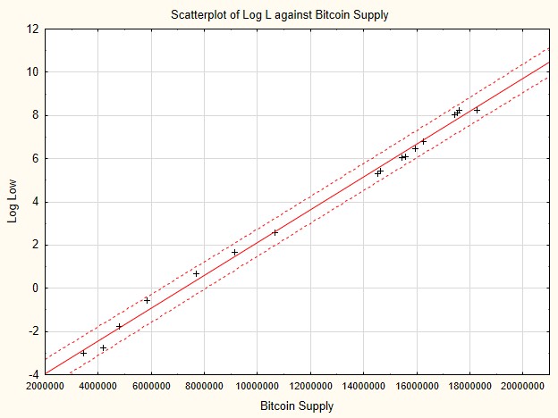
In doing so I discovered that there is a fairly strong linear relationship between the logarithm of the bitcoin price and the number of existing bitcoins at that particular moment.
All the important bitcoin bottoms are inside the 95% confidence bands (dotted lines)
With the software i use isn’t complicated to find a formula that approximate all the selected bitcoin bottoms.
This is the dataset used to compute the model:
Date
Low
Bitcoin Supply
2010/07/17
$0.05
3436900
2010/10/08
$0.06
4205200
2010/12/07
$0.17
4812650
2011/04/04
$0.56
5835300
2011/11/23
$1.99
7686200
2012/06/02
$5.21
9135150
2013/01/08
$13.20
10643750
2015/08/26
$198.19
14536950
2015/09/22
$224.08
14637300
2016/04/17
$414.61
15439525
2016/05/25
$444.63
15582350
2016/10/23
$650.32
15943563
2017/03/25
$889.08
16235100
2019/02/08
$3,350.49
17525700
2018/12/15
$3,124.00
17423175
2019/03/25
$3,855.21
17608213
2020/03/13
$3,850.00
18270000
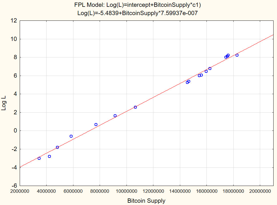
The Formula is a very simple one, a first order price regression between log(Low) and Bitcoin supply:
Where:
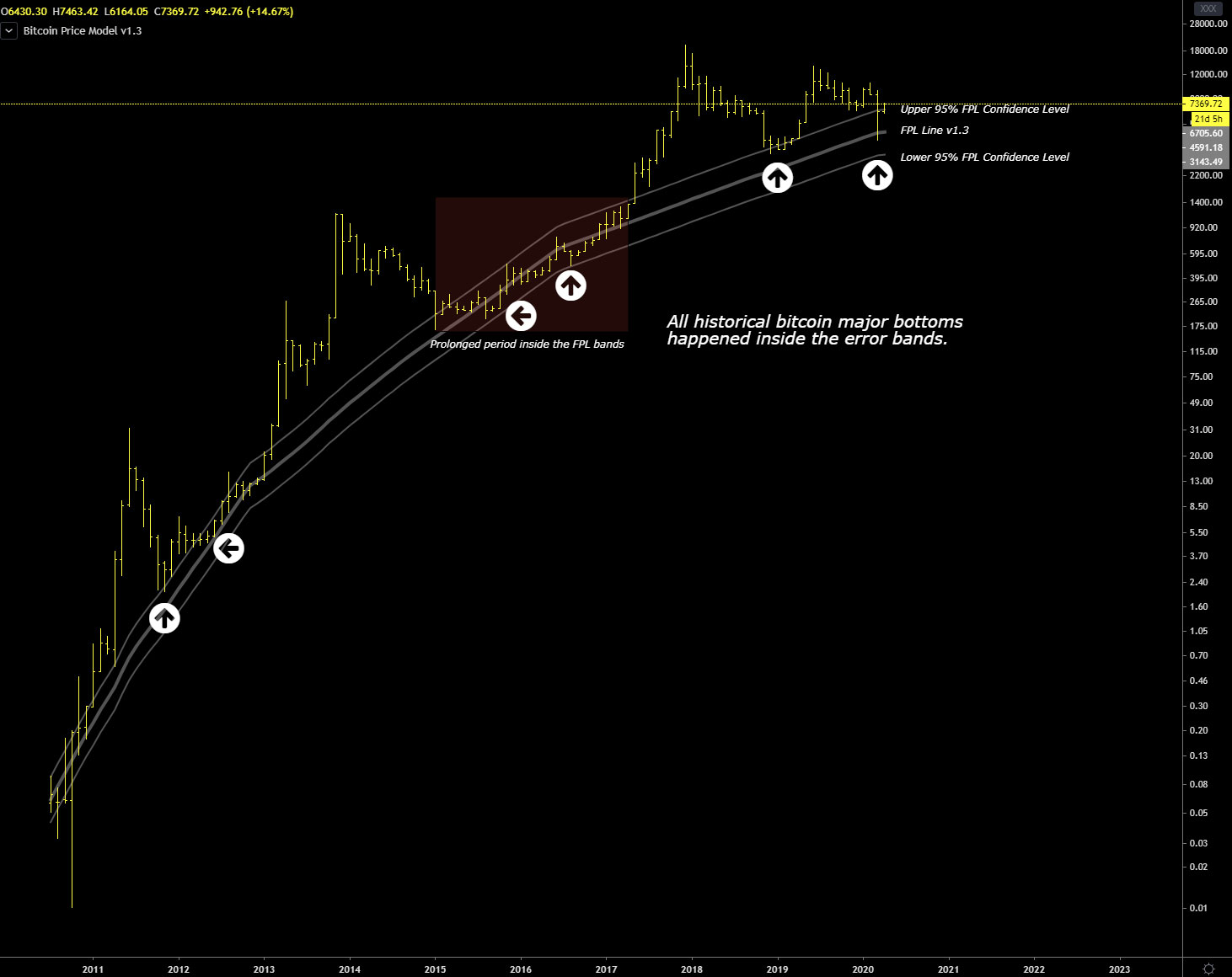
FPL = expected line where bitcoin is fairly priced
intercept = a costant
c1 = another coefficient that defines the slope of the Bitcoin supply input.
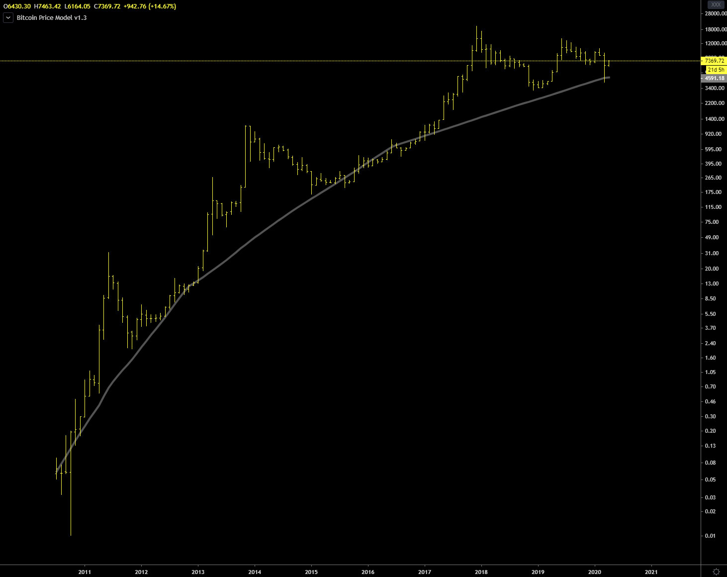
Here’s the resulting model after computing the parameters of the above formula.
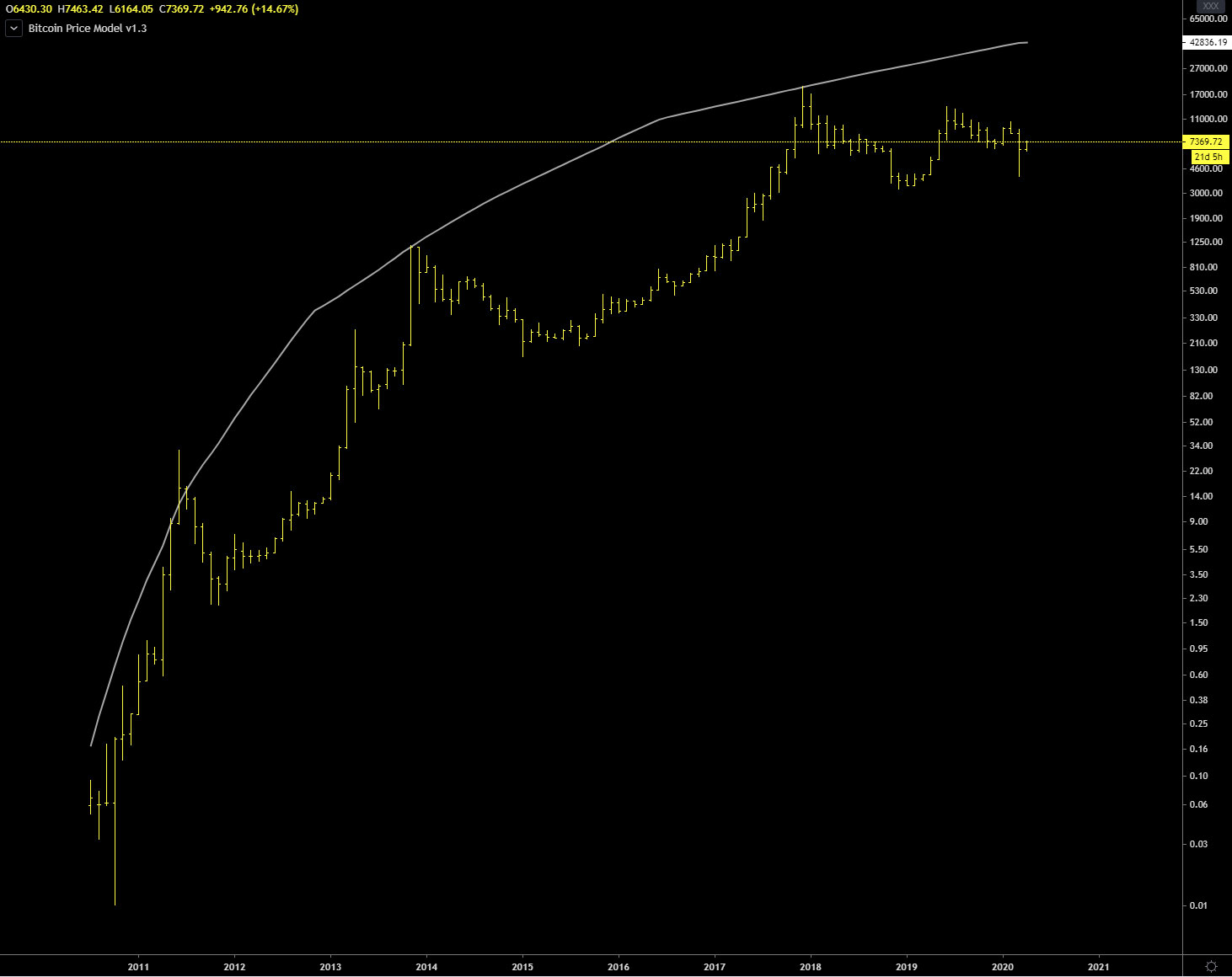
This is the new bitcoin price model “FPL Line” v1.3 applied to a monthly bitcoin/usd chart:
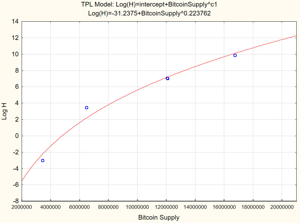
Next Step: Computing the formula for the TopLine
The formula for computing the Top is:
Where:
TopLine= is the forecasted price where the next long term top might be.
intercept = a costant
c1 = another coefficient that defines at which pow the bitcoin supply is elevated
This formula is different from the one used to compute the FPL or bottom line. I’ve seen that there is not a strong linear relationship betweel the logarithm of important Bitcoin Tops and the Bitcoin supply, so i decided to switch to the formula used for the old model and it works better.
This is the dataset used to compute the model:
Date
Price
Bitcoin Supply
2010/07/17
$ 0.05
3436900
2011/06/08
$ 31.91
6471200
2013/11/30
$ 1,163.00
12058375
2013/12/04
$ 1,153.27
12076500
2017/12/19
$ 19,245.59
16750613
Here’s the resulting model after computing the parameters of the above formula.
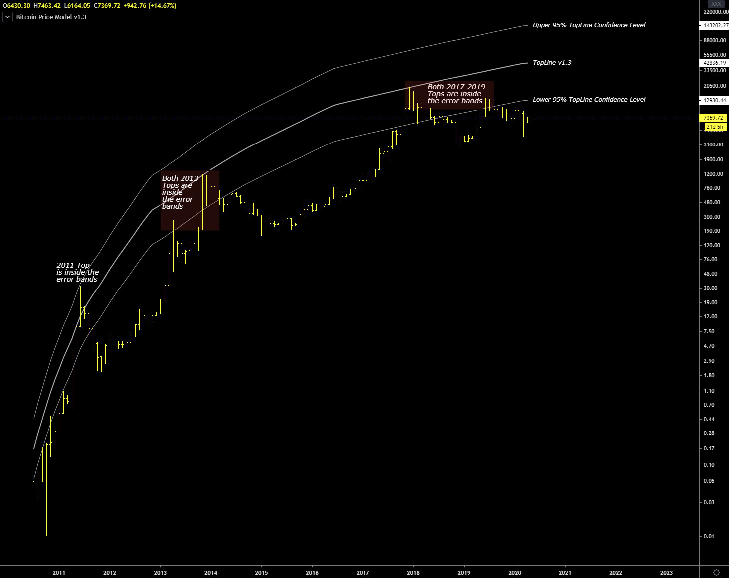
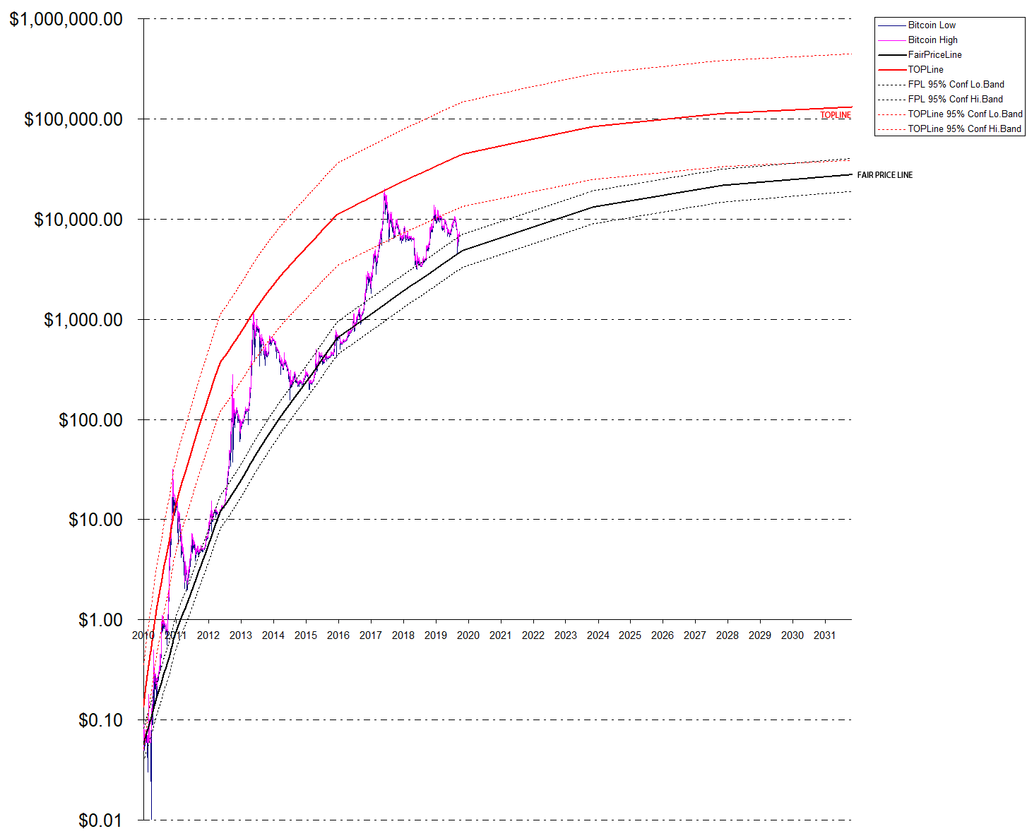
This is the new bitcoin price model “Top Line” v1.3 applied to a monthly bitcoin/usd chart:
95% Confidence Error Bands
With the indicator that i give you for TradingView i included also the error bands.
This are the error bands for the TopLine:
And for the bottom line or FPL (FairPriceLine) It is quite obvious that with fewer points available the error bands for the TopLine are wider and less accurate compared to the FPL error bands where I have more points (17 instead of 5).
TradingView Indicator
I have also included an indicator for TradingView to give you the opportunity to experience the concepts and model illustrated in this update. You can also check the code and/or modify it as you like.
On April 10th, 2020 tradingview staff decided to censor my indicator and threatened to close my account, because of this i publish here the code so you can create your own indicator by yourself.
Remember to add a “TAB” key once before stock (line 10 and 13), in the process of copying and pasting data back and forth from tradingview the tab key is gone probably because there is not a tab code in HTML.
This is a forecast up to 2032 halving, price will saturate between 27,000$ and 130,000$ with a maximum possible peak at 450,000$ in case of a strong bubble.
Conclusions
This model is clearly experimental, we will see in the future how it will behave. It is probably questionable my choice to use the existing bitcoin supply instead of using time as a main input for the model, I’m curious to know your opinion about it. Thank you.
This post is meant to be an addition to what I said earlier this year. Here we compare, in the same historical period of existence of bitcoin, Bitcoin vs other assets: us stock market indexes, US stocks of different sectors and Gold.
Let’s start with this summary table, who follow me regularly should already know the meaning of Shannon’s probability, RMS, G yield and compounded annual G yield; for all the others I refer you to the end of the article.
The data have been sorted in descending order according to Compounded Yearly Gain G.
Comparison Bitcoin vs. The rest of the world
July 17, 2010 – Dec 31, 2019
Asset
RMS or Volatility
Shannon Probability P
Daily Gain G
Compounded Yearly Gain G
Optimal Fraction of your capital to wage
Bitcoin
0.0567
0.5219
1.00087
38%
4.4%
MasterCard
0.0155
0.5265
1.0007
19%
5.3%
Visa
0.0144
0.5241
1.0006
16%
4.8%
Amazon
0.0193
0.5196
1.00057
15%
3.9%
Apple
0.0161
0.5172
1.00042
11%
3.4%
Google
0.0148
0.5167
1.00038
10%
3.3%
Microsoft
0.0143
0.5169
1.00038
10%
3.4%
Nasdaq Composite Index
0.0106
0.5179
1.00032
8%
3.6%
Standard & Poor’s 500 Index
0.0091
0.5160
1.00025
6%
3.2%
McDonald
0.0098
0.5119
1.00019
5%
2.4%
Berkshire Hathaway Inc. (W.Buffett)
0.0105
0.5112
1.00018
5%
2.2%
Pfizer
0.0115
0.5078
1.00011
3%
1.6%
Facebook
0.0226
0.5080
1.00010
3%
1.6%
Tesla
0.0318
0.5096
1.00010
3%
1.9%
JPMorgan
0.0155
0.5070
1.00010
2%
1.4%
Intel
0.0153
0.5040
1.00001
0%
0.8%
**Gold (XAUUSD)
0.0094
0.4951
0.99986
-3%
0%
*Ethereum
0.0634
0.5138
0.99974
-6%
0%
General Motors
0.0178
0.4903
0.99950
-12%
0%
General Electric
0.0164
0.4868
0.99943
-13%
0%
*Ethereum Data since Aug 7, 2015, source coinmarketcap.
**Gold since 1970 has been a bit better with +3% yearly compounded gain.
The first comparison to make is with the main competitors of bitcoin, credit cards. I’m surprised to see how good are quantitative parameters of Mastercard and Visa, on the other hand they are monopolies, perhaps that’s why the CEO of mastercard hates so much Bitcoin, he sees it as a strong threat. Even Amazon has worse parameters compared to Visa and MC.
I included only Ethereum in the comparison because in terms of market cap is second to Bitcoin, its yearly yield G is negative and i’m not surprised because I remind you that volatility reduces by far the yield G and in the case of all altcoins, not only Ethereum, the volatility reaches very high levels and therefore as an investment vehicle altcoins in general are absolutely not recommended, can eventually be considered as purely speculative assets for short-term trading.
Unfortunately for Mr.P.Schiff, in the last ten years Gold performed badly, for your curiosity i computed Gold parameters using available daily data since January 1970 and its yearly gain G or yield has been +3%, nothing exceptional, basically Gold protected you against inflation in the last fifty years but nothing more then this.
As i said 20 days ago Bitcoin volatility is dropping but it remains very high compared to other assets, despite this Bitcoin yearly compounded gain G is an astonishing +38% and it’s the best investment vehicle of the world.
Compared to other bitcoin price models this value is not much, ten years from now compounding 38% yearly bitcoin should be at around 200k usd while, for example, the stock to flow model has a forecast of 10 millions usd after 2028 halving, this is the equivalent of 144% yearly compounded gain instead of 38%.
Let me know what you think, does the stock to flow model price return appear realistic to you or not? Personally i prefer to rely on numbers and they say a clear “no” to me. This is why i’m a bit skeptic about also the bitcoin price model i developed on tradingview but i’m curious to see how it’ll end in a couple of years.
Tech Addendum
The concept of entropic analysis of equity prices is old and it was first proposed by Louis Bachelier in his “theory of speculation”, this thesis anticipated many of the mathematical discoveries made later by Wiener and Markov underlying the importance of these ideas in today’s financial markets. Then in the mid 1940’s we have had the information theory developed by Claude Shannon , theory that is applicable to the analysis and optimization of speculative endeavors and it is exactly what i’ve done just applied to bitcoin and the other assets considered in the above table, especially using the Shannon Probability or entropy that in terms of information theory, entropy is considered to be a measure of the uncertainty in a message.
To put it intuitively, suppose , at this probability, the event is certain never to occur, and so there is no uncertainty at all, leading to an entropy of 0; at the same time if the result is again certain, so the entropy is 0 here as well. When or 0.50 the uncertainty is at a maximum or basically there is no information and only noise.
Applying this entropy concept to an equity like a stock or a commodity or even bitcoin itself common values for P are 0.52 that can be interpreted as a slightly persistence or tendency to go up, this means that for example stock markets aren’t totally random and up to some extend they are exploitable, same for btc.
Knowing the entropy level of bitcoin/usd is crucial if we want to compute its main quantitative characteristics, as i explained in the technical background of my blog this process is quickly doable once you have all the formulas, the process is as follows:
To compute the Shannon Probability P you should follow these steps:
compute natural logarithm of data increments (today price / yesterday price)
compute the mean for all data increment computed in step 1
compute RMS (root mean square) of all data increments, squaring each data increment and sum all togheter
Compute price momentum probability with the formula P = (((avg / rms) – (1 / sqrt (n))) + 1) / 2 where avg = data computed in step 2, rms = data computed in step 3, n = total samples of your dataset. If the resulting probability is above 0.5 then there is positive momentum, otherwise under 0.5 negative momentum
To compute the Gain Factor G use the following formula:
G = ((1+RMS)^P*((1-RMS)^(1-P))
To compute the yearly gain G or growth just raise daily gain G to the 365th power for Bitcon or 252 for stocks (252 trading days in a year).
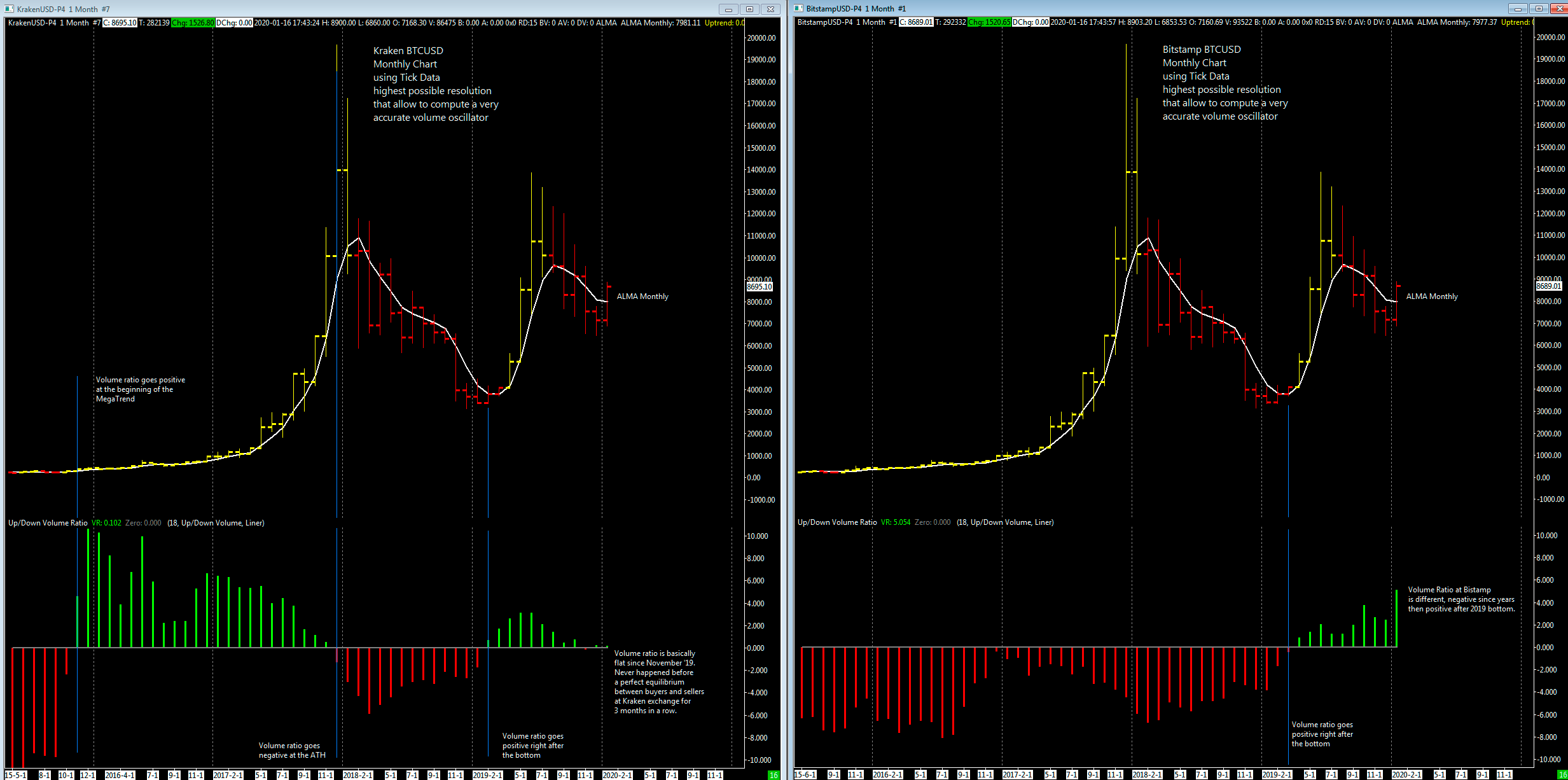
The trading platform used here is unchanged: Sierrachart 64 bit.
The big amount of tick data processed to compute this interesting volume oscillator wouldn’t be possible to do at TradingView or similar online platforms.
The “up/down Volume Ratio” oscillator is computed and smoothed using a 18 periods (18 months or 1 year and a half) linear regression moving average.
Volume made on an uptick is considered positive while if made on a downtick is negative, then the aforementioned oscillator is applied.
I added also in the chart the widely know ALMA moving average (9 periods, standard settings).
I added for comparison the same template applied to BTCUSD at Bitstamp exchange.
Volume Ratio Oscillator Kraken/Bitstamp Comparison (click to enlarge)
Very curious to see a perfectly balanced volume activity at Kraken exchange for 3 months in a row while at the Bitstamp the volume activity is unbalanced upwards.
As a positive note i can say that i don’t see any negative volume activity in either of the two exchanges considered. Said this my best guess is that the price retracement from about $13800 to $6400 was a normal correction of a bullish market and that the bear market ended on March ’19.


 , at this probability, the event is certain never to occur, and so there is no uncertainty at all, leading to an entropy of 0; at the same time if
  the result is again certain, so the entropy is 0 here as well. When
  or 0.50 the uncertainty is at a maximum or basically there is no information and only noise.