
I waited a while before updating you about the short term situation because i wanted to see if the trend confirmed by the Kama efficiency rate was good and not a false signal.
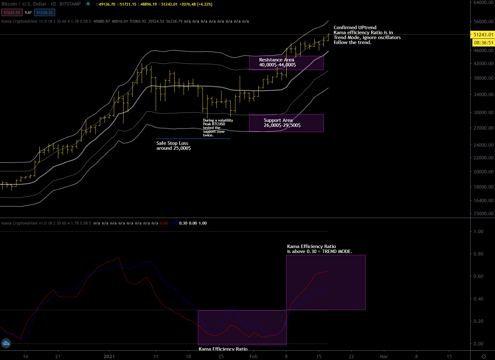
As I have said many times in the past, when the Kama average is flat there are very good resistance and support zones that define the useful space in which an asset, in this case bitcoin, moves.
Outside of these resistance zones a trend reversal is confirmed (if we break the support zone) or the continuation of the bullish trend (if we break the resistance zone).
What has happened is that bitcoin has broken the resistance zone positioned at 40-44 thousand dollars thus confirming the bullish trend. On the weekly chart the trend is strong and price remains consistently above the weekly Kama average.
Kama efficiency ratio is now in “Trend Mode” on all the main timeframes: Daily, Weekly, Monthly; therefore my outlook is strongly bullish.

Thanks again for the update.
I have a question. I have applied the kama model from the link you shared, but the support and resistance levels are always about 2k off from what you are posting in your charts. When you were getting 40-44, I was getting around 38-42. I use the same exchange as you, same time frequency, nothing seems to be different. Perhaps you have updated the model and I got some old version or is there any other explanation? Thank you!
// This source code is subject to the terms of the Mozilla Public License 2.0 at https://mozilla.org/MPL/2.0/
// © CryptoAdvisor_
//@version=2
study(“Kama CryptoAdvisor v1.0″, overlay=true)
length = input(title=”Length”, type=integer, defval=18)
fastLength = input(title=”Fast EMA Length”, type=integer, defval=2)
slowLength = input(title=”Slow EMA Length”, type=integer, defval=30)
//LOW
mom = abs(change(low, length))
volatility = sum(abs(change(low)), length)
// Efficiency Ratio
er = volatility != 0 ? mom / volatility : 0
fastAlpha = 2 / (fastLength + 1)
slowAlpha = 2 / (slowLength + 1)
// KAMA Alpha
sc = pow((er * (fastAlpha – slowAlpha)) + slowAlpha, 2)
kama = 0.0
kama := sc * low + (1 – sc) * nz(kama[1])
//HIGH
mom1 = abs(change(high, length))
volatility1 = sum(abs(change(high)), length)
// Efficiency Ratio
er1 = volatility1 != 0 ? mom1 / volatility1 : 0
// KAMA Alpha
sc1 = pow((er1 * (fastAlpha – slowAlpha)) + slowAlpha, 2)
kama1 = 0.0
kama1 := sc1 * high + (1 – sc1) * nz(kama1[1])
//Price Bands
show_P1 = input(true, type=bool, title=”Show Kama with computed volatility(RMS)”)
periods = input(title=”RMS Periods”, type=integer, defval=60)
t = input(title=”Time for price bands”, type=integer, defval=4)
rms_h=pow(sum(pow(log(high/high[1]),2),periods)/periods,0.5)
rms_l=pow(sum(pow(log(low /low[1]),2), periods)/periods,0.5)
plot(show_P1 ? (kama+kama1)/2 : na, color=gray, title=”MidPoint”, linewidth=3, transp=0)
plot(show_P1 ? kama*exp(-rms_l*1*sqrt(t)) : na, color=gray, title=”-1 dev.”, linewidth=1, transp=0)
plot(show_P1 ? kama1*exp(rms_h*1*sqrt(t)) : na, color=gray, title=”+1 dev.”, linewidth=1, transp=0)
plot(show_P1 ? kama*exp(-rms_l*2*sqrt(t)) : na, color=gray, title=”-2 dev.”, linewidth=2, transp=0)
plot(show_P1 ? kama1*exp(rms_h*2*sqrt(t)) : na, color=gray, title=”+2 dev.”, linewidth=2, transp=0)
show_P2 = input(false, type=bool, title=”Show Kama with fixed volatility using DELTA parameter”)
delta = input(1.78,”Delta High”,step=0.01)
deltal= input(0.58,”Delta Low”,step=0.01)
plot(show_P2 ? (kama+kama1)/2 : na, color=gray, title=”MidPoint”, linewidth=2, transp=0)
plot(show_P2 ? kama*deltal : na, color=gray, title=”-1 dev.”, linewidth=1, transp=0)
plot(show_P2 ? kama1*delta : na, color=gray, title=”+1 dev.”, linewidth=1, transp=0)
//plot(show_P2 ? kama*(deltal*2) : na, color=gray, title=”-2 dev.”, linewidth=2, transp=0)
//plot(show_P2 ? kama1*(delta*2) : na, color=gray, title=”+2 dev.”, linewidth=2, transp=0)
//EFF RATIO
show_SNR = input(false, type=bool, title=”Show Kama Efficiency Ratio”)
SNR_Smoothing = input(5,”EMA periods smoothing SNR”,step=1)
plot(show_SNR ? ema(er,SNR_Smoothing) : na, color=red, title=”SNR Ratio Low of the bar”)
plot(show_SNR ? ema(er1,SNR_Smoothing) : na, color=blue, title=”SNR Ratio High of the bar”)
plot(show_SNR ? 0.30 : na, color=white, title=”0.60 thresold”, linewidth=1, transp=80)
plot(show_SNR ? 0.00 : na, color=white, title=”zeroline”, linewidth=1, transp=80)
plot(show_SNR ? 1.00 : na, color=white, title=”upper limit”, linewidth=1, transp=80)
//Paint Bars
showcolors1 = input(false, type=bool, title=”Strong/Flat Market”)
strong_market = ema(er,SNR_Smoothing) > 0.80 or ema(er1,SNR_Smoothing) > 0.80 and showcolors1==true
flat_market = ema(er1,SNR_Smoothing) < 0.30 or ema(er1,SNR_Smoothing) < 0.30 and showcolors1==true
barcolor(showcolors1 and flat_market ? red : na)
barcolor(showcolors1 and strong_market ? white : na)
I updated the model, look for “Kama CryptoAdvisor 1.0” or “Kama 1.0” by “CryptoAdvisor_” (new username at tradingview) https://www.tradingview.com/u/CryptoAdvisor_
You should find the indicator in my published script
https://www.tradingview.com/u/CryptoAdvisor_/#published-scripts
Is it possible to determine resistance zones of the trend mode?
yes but they would not be reliable because the tendency is not flat. you could make some estimates on the target of the trend supposing that hardly the duration of a trend exceeds the 25-30 bars without first making a correction or a phase of laterality, but this indicator can’t do this.
Hello! Watching your analysis for several years now, thank you for your work. Do you think the current price action is just a correction and we’ll see more highs in upcoming weeks or that the long term (3-4yrs) top has been made?
the top has not been made IMO, this is only a correction, aniway is better to proceed one step at a time, let’s see if the first support zone will work, it is located between 39 and 44 thousand dollars.