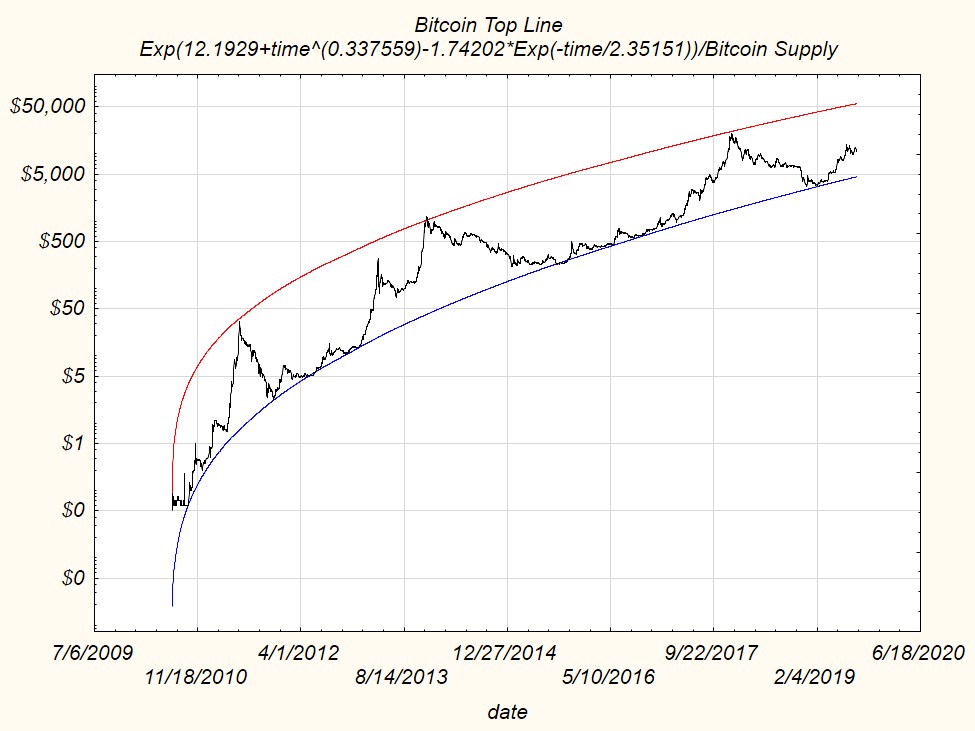
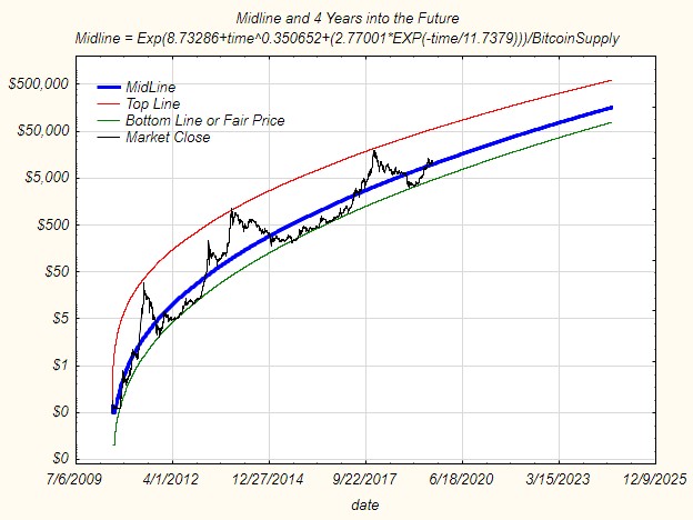
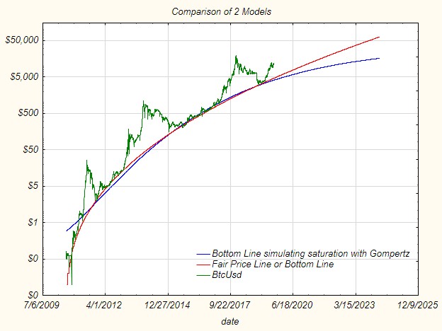
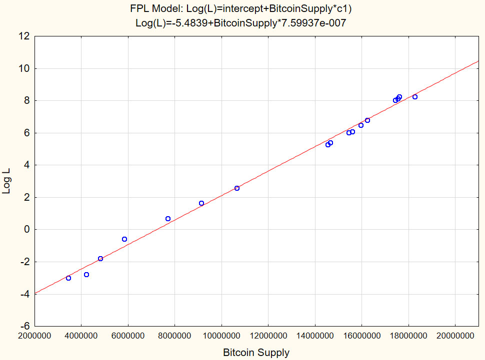
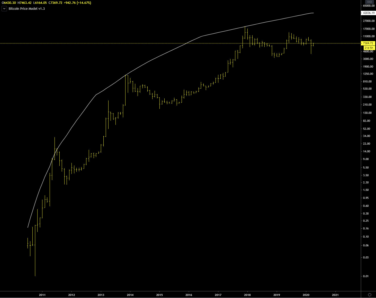
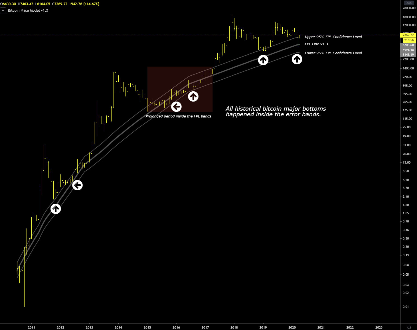
If the “Two-Phase Power Law” model defines the floor (Fair Value), a complementary equation defines the ceiling: the Peak Envelope.
To understand where price may go in this cycle, we must analyze two opposing dynamics that evolve over time:
- The deceleration of the rise (Slope Decay).
- The contraction of the bubble (Peak Envelope Decay).
1. The Mathematics of the Rise (Slope Decay)
One of the main flaws of fixed 4-year models is the assumption that every cycle is identical in time. The data show the exact opposite and the speed at which price rises from bottom to top is decreasing according to an inverse power law.
By analyzing past cycles, we obtain the following formula for the slope (rate of ascent in logarithmic terms):
Slope = 14.68 × n^(-2.17) decades/year
Where n is the cycle number.
| Cycle | Length (days) | True Slope (Dec/Year) | Slope Model |
|---|---|---|---|
| 2 | 295 | 3.291 | 3.267 |
| 3 | 742 | 1.358 | 1.356 |
| 4 | 1068 | 0.704 | 0.727 |
| 5 | 1061 | 0.459 | 0.448 |
| 6 | ? | ~0.21 so far | 0.302 |
What does this mean? In 2013 (Cycle 3), the market was rising at a crazy speed (1.35 decades per year). For Cycle 6, the model predicts a slope of 0.302.
It is like saying: “The Ferrari has turned into a freight train. It is still powerful, but it takes much longer to reach its destination.”.
The “Slope” (velocity) in this model tells us how many powers of 10 the price rises by every year:
Slope 3.0 = Price multiplies by 1,000 every year.
Slope 1.0 = Price multiplies by 10 every year.
Slope 0.3 = Price doubles every year.
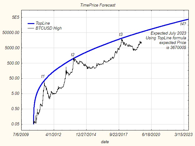
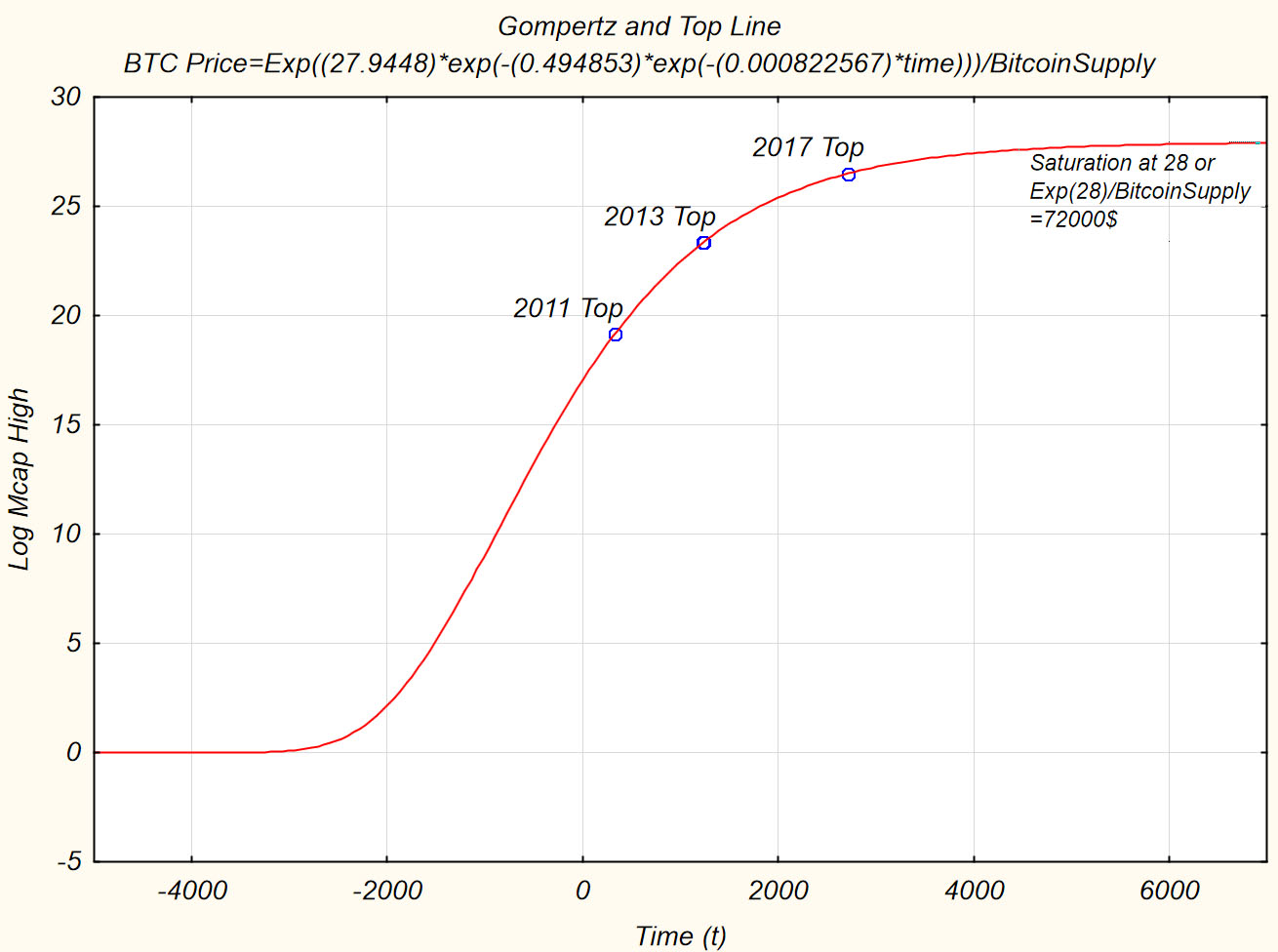
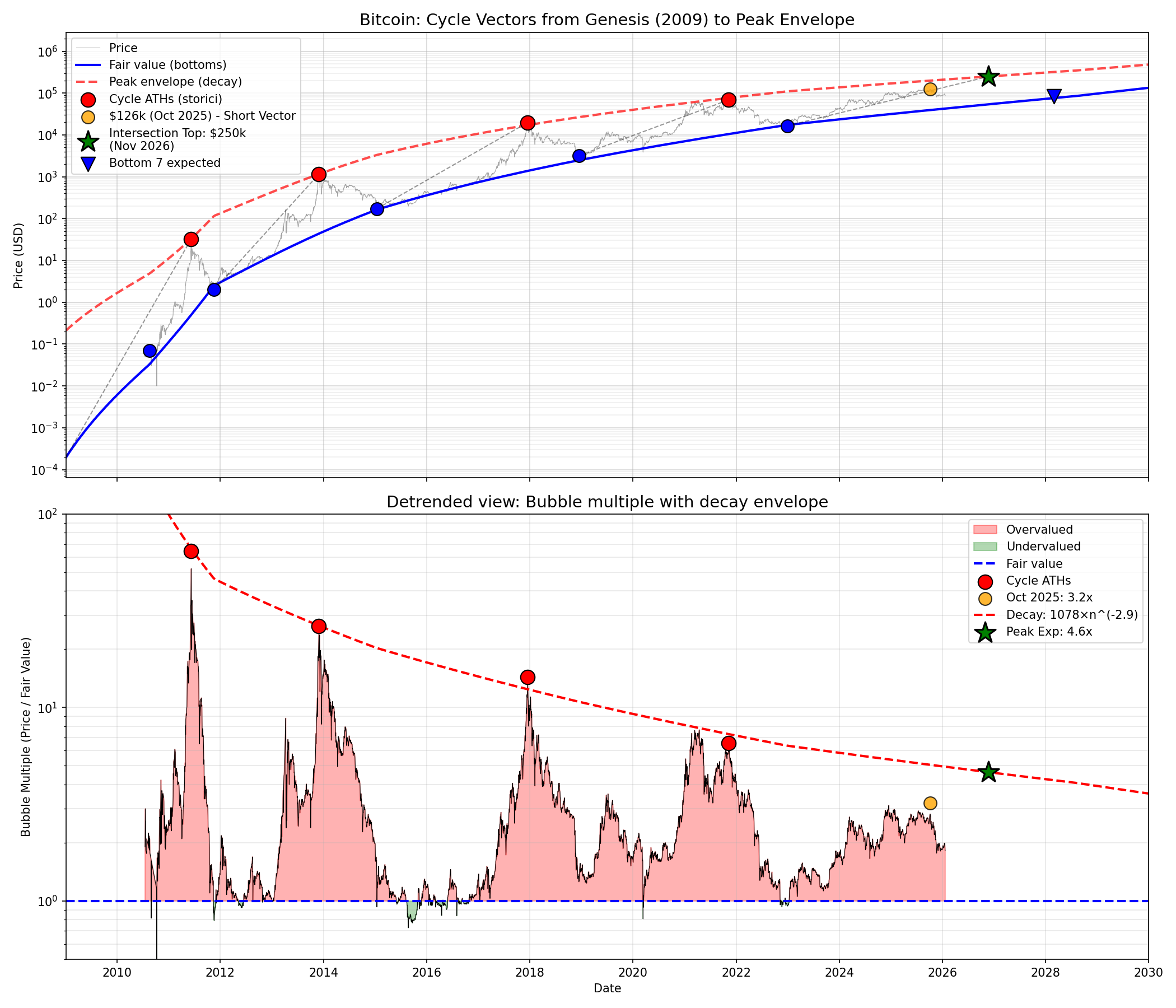
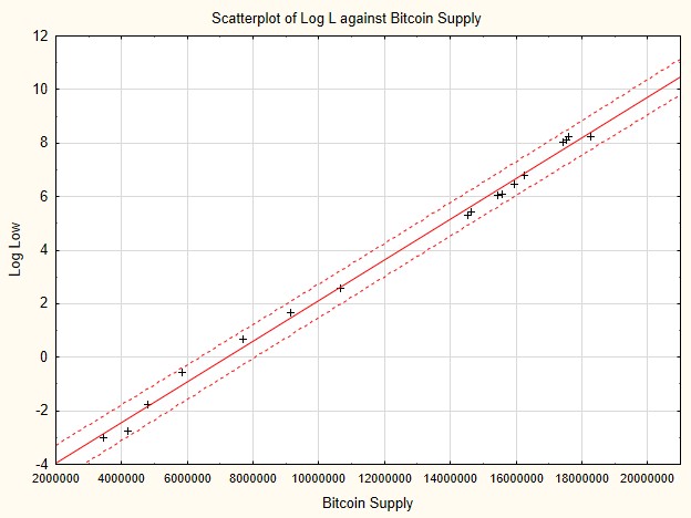
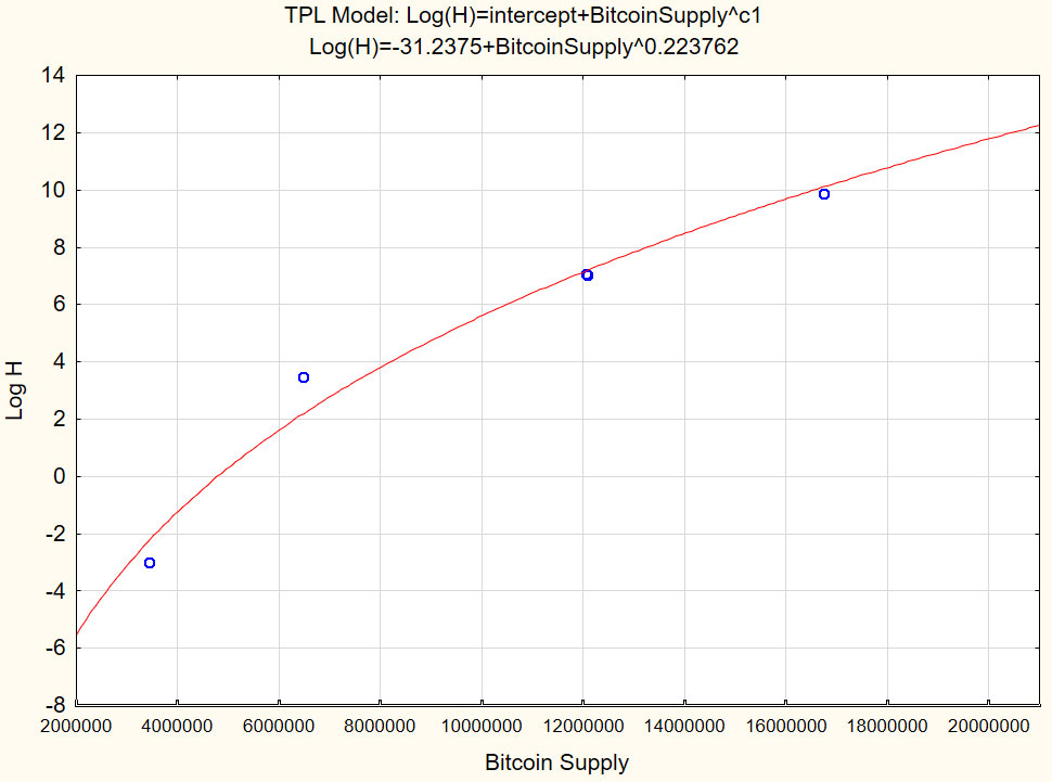
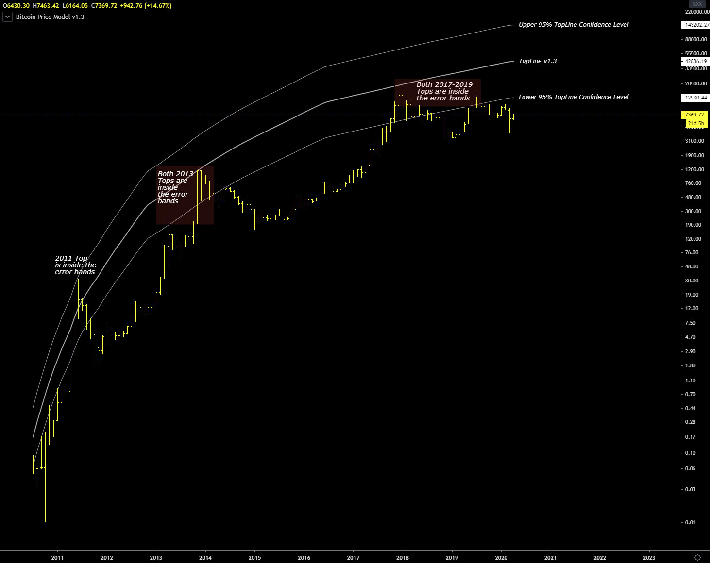
2. The Peak Envelope
While price rises more slowly, the bubble multiple (how far above Fair Value we are willing to pay) is collapsing.
- In 2013 we paid 25× Fair Value.
- In 2021 we paid about 7× Fair Value.
- In this cycle the ceiling (Envelope) will fall even further to an expected value of 4.7x
We modeled this decay using an inverse logarithmic curve that connects historical peaks.
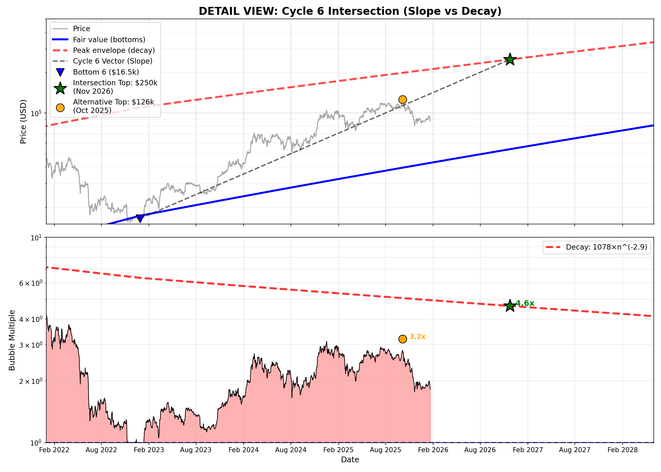
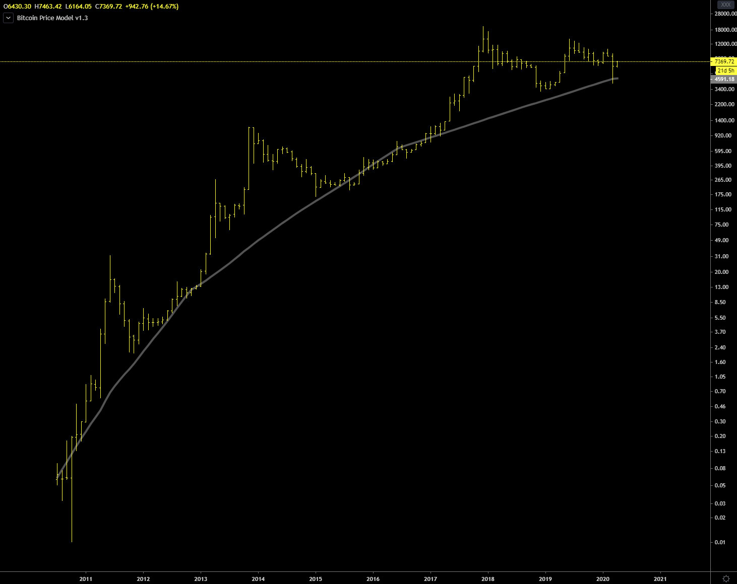
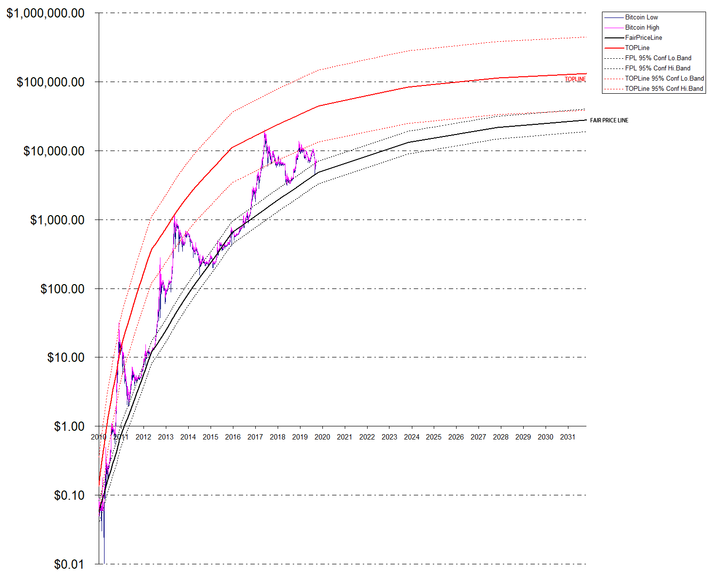
3. The ‘Self-Consistent’ Projection at ~$250k
Instead of guessing a date, I wrote an iterative algorithm (in Python) that searches for the geometric intersection between two forces:
- The Upward thrust: the line starting from the bottom ($16,500) with the Cycle 6 slope (0.302).
- The Ceiling: the Peak Envelope curve declining over time.
The point where these two lines collide is the cycle top. (check below images)
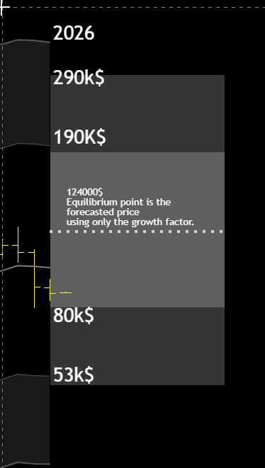
Model Result (Baseline):
- Peak date window: from November 2026 to April 2027.
- Price: ~$250,000
- Multiple: about 4.7× above Fair Value at that time
This scenario represents historical continuity. A longer cycle than previous ones, extending beyond the usual 4-year pattern, allowing price to grow until the bubble multiplier stops it.
A November 2026 top may be optimistic, the date can shift to April 2027 due to slope uncertainty.
=== FIT ===
slope = 14.6835 × n^(-2.17) decades/year
Std residuals: 0.0242 decades/year
=== SLOPE Cycle 6 ===
Forecasted value: 0.302 decades/year
Error (1σ): ±0.024 decades/year
+1σ: 0.326 decades/year
-1σ: 0.278 decades/year
| Scenario | Slope dec/year | Top Date | Top Price | Bottom Date | Bottom Price |
| -1σ | 0.278 | 2027-03-31 | $ ~250,000 | 2029-01-24 | $84,770 |
| Mid | 0.302 | 2026-11-27 | $ ~250,000 | 2028-07-31 | $83,800 |
| +1σ | 0.326 | 2026-08-13 | $ ~250,000 | 2028-03-02 | $76,000 |
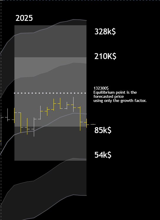
4. Alternative Scenario: The ‘Short Top’ at $126k
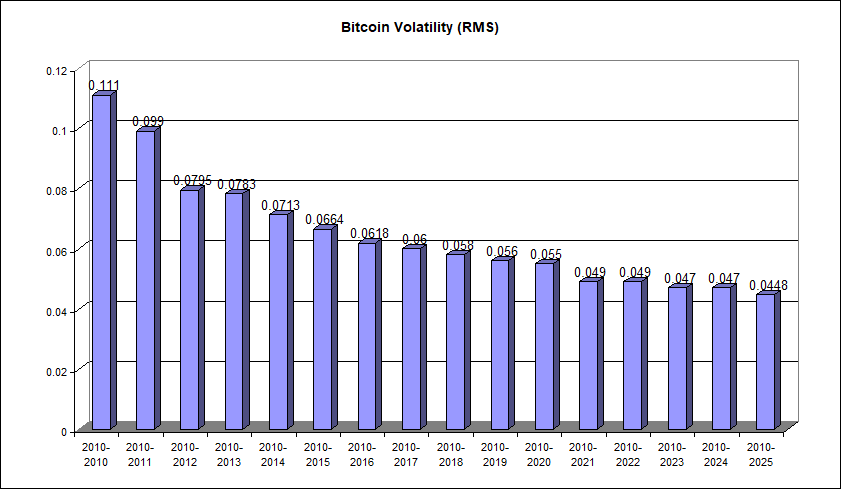
The model is sensitive to volatility compression. If the peak envelope decays faster than the historical average, the intersection happens much earlier.
In this contraction scenario the top has already been done:
- Peak date: 6 October 2025
- Price: $126,000
- Implication: the market would have become efficient too early. Bitcoin would behave like a mature asset, with short cycles and low multiples, eliminating extreme euphoria phases.
If the last October top at $126,000 is confirmed as top of cycle 7 then it’s very easy to compute date and price of the bottom, $54,000 by December 2026 (fair price of my 2 phases price model) resulting in a perfect 4 year cycle, 4 years between November 2022 bottom and December 2026.
Conclusion
The model establishes $250,000 by late 2026 (with a potential extension into early 2027) as the natural geometric output”. In this baseline scenario the cycle’s ascent perfectly intersects the historical ‘Peak Envelope,’ maintaining the balance between price momentum and the decay of bubble multiples.
Conversely, a peak at $126,000 in October 2025 would not invalidate the model, but would signal accelerated market saturation. This ‘short top’ scenario implies that the market is no longer willing to pay the excessive premiums of the past.
It effectively suggests that Bitcoin’s valuation will be capped at approximately 2x its intrinsic Fair Value during each boom-bust cycle. Such a move would mark the definitive transition from a hyper-volatile speculative instrument to a mature, low-volatility asset.


 , at this probability, the event is certain never to occur, and so there is no uncertainty at all, leading to an entropy of 0; at the same time if
  the result is again certain, so the entropy is 0 here as well. When
  or 0.50 the uncertainty is at a maximum or basically there is no information and only noise.