Why a simple power law fails, and how a sigmoid transition model captures Bitcoin’s evolution from chaotic experiment to mature asset

January 2026 · btctrading.blog

---

Key Findings

• Predicted bottom for Cycle 7 (2025): $85,197 (current low: $80,537, difference: -5.5%)
• 95% Confidence Interval: $43,697 – $138,437
• Phase Transition: Bitcoin’s price exponent shifted from b≈7 (early) to b≈10 (mature) around 2011
• Model Validation: R² = 0.997, outperforms simple power law on leave-one-out cross-validation
• Right-click on any image → “Open image in new tab” to enlarge

---

The Problem with Simple Power Laws

For years, Bitcoin analysts have observed that cycle bottoms follow a power law pattern. The model is elegant: each successive cycle bottom follows the formula Price = a × n^b, where n is the cycle number and b is a constant exponent. When applied to the four “market era” bottoms (2011, 2015, 2018, 2022), this model achieves an impressive R² of 0.998.

But Bitcoin didn’t begin in 2011. What happens when I include the true origins, the mining cost at genesis (January 2009) and the first exchange price on Mt.Gox (August 2010)?

The model collapses. A single power law cannot span from $0.0001 to $15,474 while maintaining predictive accuracy. The early points pull the fit in one direction, the recent points in another, and the result is a compromised model that fits nothing well.

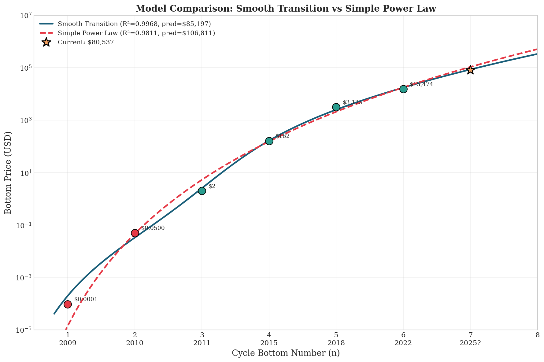Figure 1: A simple power law (dashed red) cannot accurately fit both early and recent data points. The smooth transition model (solid blue) captures the phase shift in Bitcoin’s evolution.

---

The Core Insight: Normalizing Time

Most Bitcoin models plot price against calendar time, days or years since genesis. But this introduces a distortion: early cycles were short and chaotic, later cycles are longer and more stable.

By indexing bottoms by cycle number (n=1, 2, 3…) rather than calendar time, we normalize this distortion. Each cycle becomes one unit, regardless of its duration in days. This allows the underlying growth pattern to emerge more clearly.

---

The Two-Phase Hypothesis

The insight is that Bitcoin in 2009 was a fundamentally different system than Bitcoin in recent years.

Early Phase (2009-2010):

• Handful of participants
• No real market or price discovery
• High noise, low signal
• Dominated by technical curiosity

Mature Phase (2012+):

• Functioning exchanges and price discovery
• Growing user base (thousands → millions over time)
• Increasingly liquid markets
• Later: institutional interest, CME futures (2017), spot ETFs (2024)

The transition between these phases was gradual, centered around 2011 when Bitcoin experienced its first real boom/bust cycle and Mt.Gox established genuine price discovery.

If the underlying system changed, why would we expect a single mathematical relationship to describe both eras? The answer is: we shouldn’t, instead we need a model that allows the exponent itself to evolve over time.

---

The Smooth Transition Model

Rather than a fixed exponent b we allow the exponent to transition smoothly from an early-phase value (b₁) to a mature-phase value (b₂) via a sigmoid function:

Price = a × n^b(n)

Where the exponent evolves:
b(n) = b₁ × (1 - σ) + b₂ × σ

And σ is a sigmoid transition:
σ(n) = 1 / (1 + e^(-k×(n-3)))

Fitted Parameters:
a  = 0.000196     # scale factor
b₂ = 10.22        # mature phase exponent (fitted)
b₁ = 7.0          # early phase exponent (fixed)
k  = 2.0          # transition speed (fixed)
n₀ = 3            # transition point (fixed at 2011)

The key innovation is reducing free parameters to just two by fixing the others at historically reasonable values. This prevents overfitting and produces a model that generalizes well to unseen data.

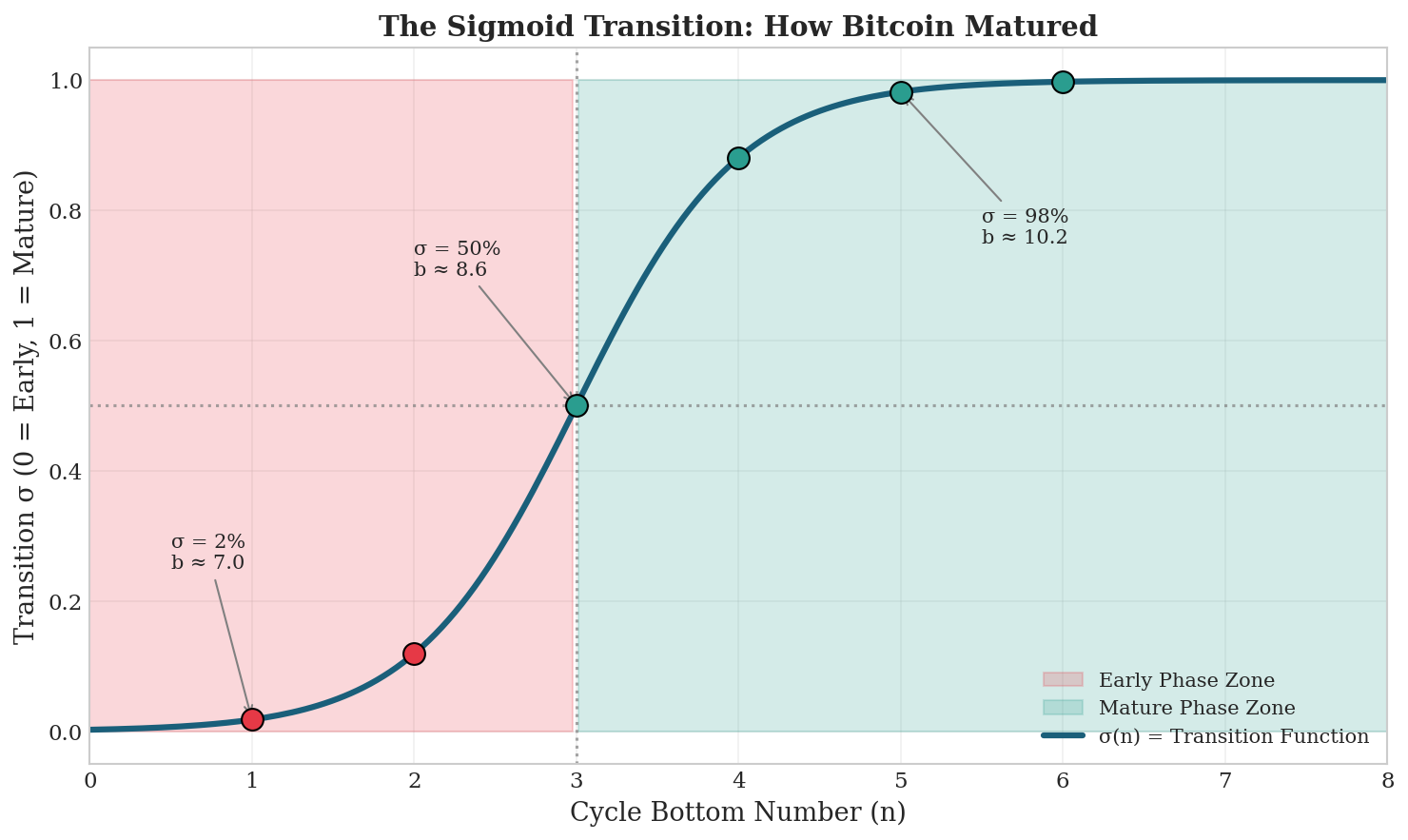Figure 2: The sigmoid function σ(n) controls the transition from early-phase dynamics (red zone) to mature-phase dynamics (green zone). At n=3 (2011), the system is exactly halfway through the transition.

---

Results and Predictions

The model achieves an excellent fit across all six historical data points spanning eight orders of magnitude in price:

n	Date	Event	Actual	Predicted	Error
1	Jan 2009	Mining cost at genesis	$0.0001	$0.0002	+106%
2	Aug 2010	Mt.Gox first trades	$0.05	$0.033	-34%
3	Nov 2011	First cycle bottom	$1.99	$2.52	+27%
4	Jan 2015	Second cycle bottom	$162	$164	+1%
5	Dec 2018	Third cycle bottom	$3,125	$2,495	-20%
6	Dec 2022	Fourth cycle bottom	$15,474	$17,410	+13%
7	2025?	Fifth cycle bottom	$80,537*	$85,197	-5.5%

*Current cycle low as of January 2026

Note that errors are larger in the early phase (n=1,2,3). This is expected, the model weights these points less because early prices came from thin, illiquid markets with few participants, making them inherently less reliable as reference points.

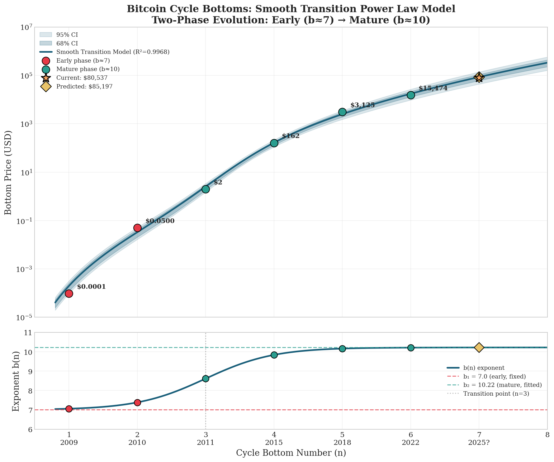Figure 3: The smooth transition model with bootstrap confidence intervals. The upper panel shows price predictions; the lower panel shows how the exponent b(n) evolves from ~7 to ~10 across the transition.

---

Model Validation: Why This Isn’t Overfitting

A critical challenge with small datasets (we have only 6 points) is distinguishing genuine patterns from overfitting. We addressed this through three approaches:

1. Parameter Parsimony

The full model has 4 parameters (a, b₁, b₂, k), but we fix 3 of them at historically reasonable values, leaving only 2 free parameters (a and b₂). This gives us 4 degrees of freedom, twice as many as a model that fits all parameters.

2. Leave-One-Out Cross-Validation

We tested model stability by removing each data point, refitting, and predicting the held-out point:

Model	Parameters	LOO MAPE	Stability
Simple Power Law	2	80%	0.26
Smooth Transition (simplified)	2	48%	0.09
Smooth Transition (full)	4	1568%	1.02

The full 4-parameter model showed catastrophic instability, removing a single point caused predictions to vary by over 1000%. The simplified model maintained reasonable predictions regardless of which point was removed.

3. Information Criteria

AIC and BIC are standard statistical measures that balance goodness of fit against model complexity, they penalize models for having too many parameters. Lower values indicate a better trade-off. Both metrics favor the simplified smooth transition model over alternatives (see Appendix A.2 for values).

---

Price vs. Adoption: Two Parallel Sigmoids

If the two-phase model reflects Bitcoin’s maturation, we should see similar patterns in adoption metrics. We compared price dynamics to the growth of unique addresses with non-zero balance:

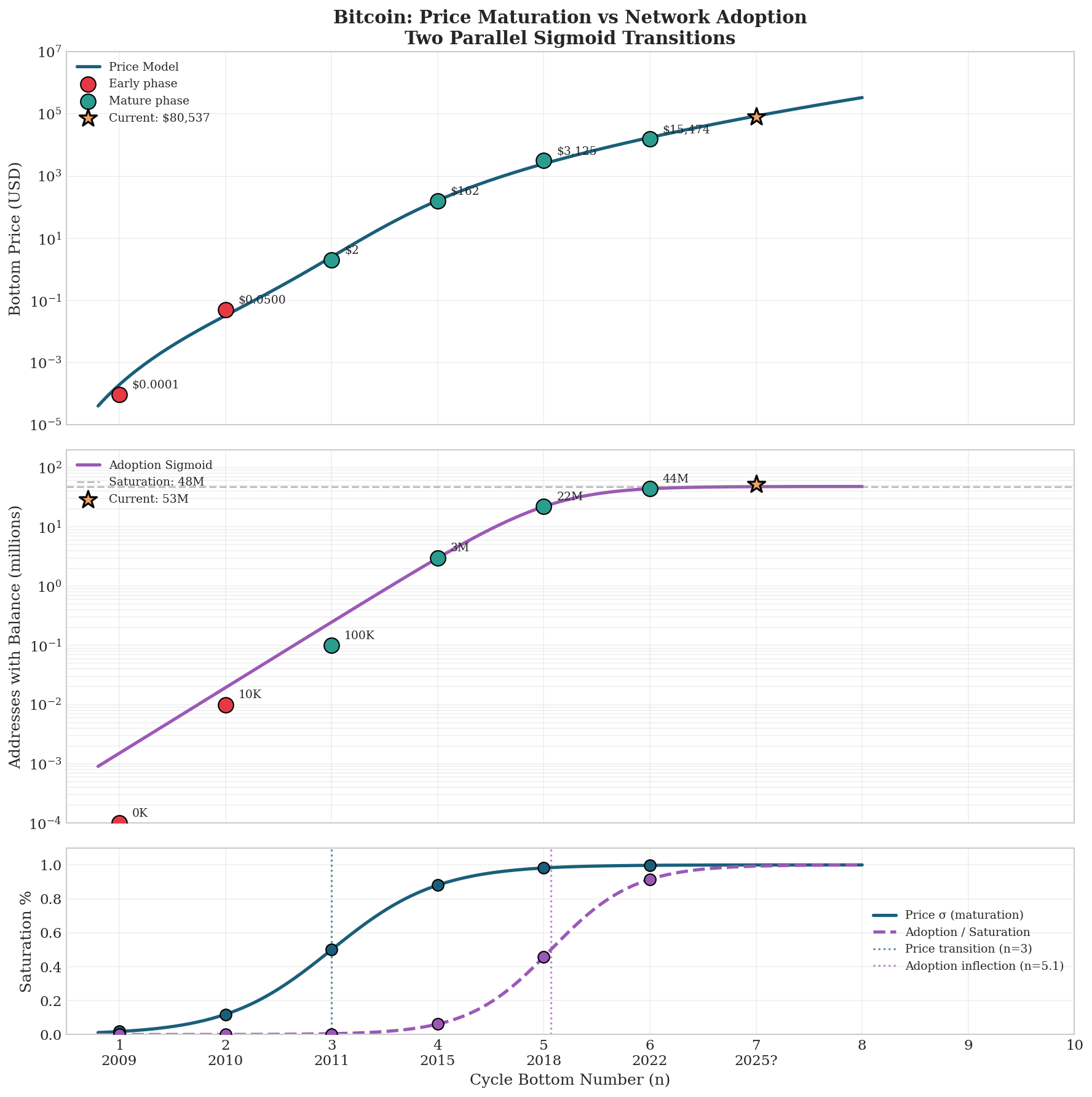Figure 4: Price maturation (blue) preceded adoption saturation (purple) by approximately two cycles. The bottom panel shows both sigmoid curves normalized to their saturation values.

A striking finding: price maturation preceded adoption by roughly 2 cycles. When the price exponent was already 88% of the way to its mature value (n=4, 2015), adoption was only at 6% of saturation. This lag suggests that price dynamics were driven by forward-looking market behavior, rather than current user numbers.

> The price didn’t wait for mass adoption, it anticipated it. This is typical of early-stage growth assets: markets price in expected future utility, not just current usage. Amazon and Tesla showed similar patterns where valuation ran ahead of fundamentals for years.

---

What “Saturation” Really Means

A common concern: if the model shows “saturation,” does that mean Bitcoin’s growth is over?

No. The saturation in our model refers to the exponent, not the price. The exponent stabilizing at b≈10 means the rate of growth acceleration has stabilized, not that growth has stopped.

Consider the analogy with internet adoption:

• Internet users saturated at ~5 billion (the sigmoid flattened)
• But internet value continues to grow: e-commerce, streaming, AI, etc.

Similarly, Bitcoin can transition from “growth driven by new users” to “growth driven by per-user value accumulation” (store of value, inflation hedge).

Future Bottom Predictions

Cycle	Est. Year	Predicted Bottom
n=7	2025	$85,197
n=8	2029	$334,210
n=9	2033	$1,114,372
n=10	2037	$3,271,856

These are bottoms, not peaks. The model suggests Bitcoin cycle bottoms could exceed $1 million within the next decade, though extrapolation this far carries substantial uncertainty.

---

Implications for Volatility

Historical drawdowns from peak to bottom have decreased with each cycle:

Cycle	Drawdown
1→2	-93%
2→3	-84%
3→4	-77%
4→5	-75%
5→6?	-36%*

*If $80,537 holds as the cycle bottom

The pattern suggests exponent saturation correlates with volatility compression. As Bitcoin matures, we should expect continued dampening of cycle amplitudes — fewer 10× gains, but also fewer -80% crashes.

---

Conclusions

1. Bitcoin underwent a phase transition from a chaotic early system (b≈7) to a mature market (b≈10), roughly centered on 2011.

2. Simple power laws fail because they cannot capture this structural change. The smooth transition model succeeds by allowing the exponent to evolve.

3. Model simplification beats complexity. Fixing parameters at historically reasonable values (rather than fitting everything) produces more robust predictions.

4. The current cycle bottom (~$80,537) is consistent with the model, falling within 1σ of the prediction ($85,197).

5. Future bottoms should continue rising at approximately n^10, implying potential million-dollar bottoms within 10-15 years.

6. Saturation of the exponent doesn’t mean death of growth, it means Bitcoin’s growth dynamics have matured, not that growth has stopped.

---

Technical Appendix

A.1 Data Sources

n	Date	Price	Source
1	Jan 3, 2009	$0.000095	Mining cost: 80W CPU @ $0.10/kWh
2	Aug 17, 2010	$0.05	Mt.Gox early trading
3	Nov 18, 2011	$1.99	TradingView
4	Jan 14, 2015	$162.00	TradingView
5	Dec 15, 2018	$3,124.51	TradingView
6	Dec 28, 2022	$15,473.78	TradingView

A.2 Model Selection Statistics

Model	k	R²	AIC	BIC	LOO MAPE
Simple Power Law	2	0.9811	-7.25	-7.66	80.1%
Smooth Transition (simplified)	2	0.9968	-17.92	-18.34	47.8%
Smooth Transition (full)	4	0.9968	-13.89	-14.72	1568%

A.3 Python Implementation

import numpy as np
from scipy.optimize import minimize

# Data
n_hist = np.array([1, 2, 3, 4, 5, 6])
bottom_hist = np.array([0.000095, 0.05, 1.99, 162, 3124.51, 15473.78])
log_bottom = np.log10(bottom_hist)

# Fixed parameters
B1_FIXED = 7.0
K_FIXED = 2.0
TRANS_POINT = 3

# Model
def smooth_transition(params, n):
    log_a, b2 = params
    sigma = 1 / (1 + np.exp(-K_FIXED * (n - TRANS_POINT)))
    b = B1_FIXED * (1 - sigma) + b2 * sigma
    return log_a + b * np.log10(n)

# Weights (n²)
weights = (n_hist**2) / np.sum(n_hist**2)

# Fitting
def objective(params):
    pred = smooth_transition(params, n_hist)
    return np.sum(weights * (log_bottom - pred)**2)

result = minimize(objective, [-4, 10], method='Nelder-Mead')
popt = result.x

# Predict cycle 7
pred_7 = 10**smooth_transition(popt, np.array([7]))[0]
print(f"Predicted bottom n=7: ${pred_7:,.0f}")

A.4 Limitations

• Small sample size: With only 6 data points, statistical power is limited
• Definition ambiguity: What constitutes a “cycle bottom” is somewhat subjective
• Non-stationarity: The Bitcoin system continues to evolve
• Black swan events: Regulatory changes or technological failures could invalidate the model
• Extrapolation risk: Long-term predictions carry substantial uncertainty

A.5 Transition Point Sensitivity Analysis

We tested whether the choice of transition point (n=3, corresponding to 2011) was optimal or arbitrary:

Transition Point	R²	MAPE	b₂	Pred n=7	Error
n=2 (2010)	0.9923	48.9%	11.00	$91,488	-12.0%
n=2.5	0.9959	31.1%	10.62	$86,720	-7.1%
n=3 (2011)	0.9968	33.6%	10.22	$85,197	-5.5%
n=3.5	0.9908	71.0%	9.85	$87,381	-7.8%
n=4 (2015)	0.9754	181.7%	9.51	$93,490	-13.9%
n=4.5	0.9517	386.9%	9.22	$105,024	-23.3%
n=5 (2018)	0.9239	708.6%	9.05	$128,748	-37.4%

Result: n=3 is optimal on both R² and prediction accuracy. Moving the transition later (n=4 or n=5) causes dramatic degradation in fit quality.

Interpretation: The phase transition occurred when Bitcoin transitioned from “experiment” to “market”, the 2011 cycle (first real boom/bust with Mt.Gox), not when it became “mainstream” in 2015-2018. By n=4, the mature-phase dynamics were already established.

---

This is not financial advice. Past performance does not guarantee future results.

---

Part II: Cycle Dynamics and Mean Reversion

From fair value to peak envelope, slope decay, and the Ornstein-Uhlenbeck framework

February 2026 · btctrading.blog

---

The Peak Envelope: Bubble Decay

While the fair value model describes cycle bottoms, Bitcoin’s peaks follow a parallel pattern: bubble multiples decay geometrically with each cycle.

For each historical top, we calculate the “bubble multiple” as peak price divided by fair value at that moment:

Cycle	Date	Peak Price	Fair Value	Multiple	Model
2	Jun 2011	$31.50	$0.52	60.6x	59.8x
3	Nov 2013	$1,242	$46	27.0x	24.8x
4	Dec 2017	$19,804	$2,011	9.8x	10.3x
5	Nov 2021	$68,997	$15,891	4.3x	4.3x

The decay follows a power law:

Multiple = 1078 × n^(-2.87)

This creates an upper boundary (the red dashed line) that compresses toward fair value over time. The implication: future bubbles will be progressively milder. By cycle 10, the expected multiple drops below 2x.

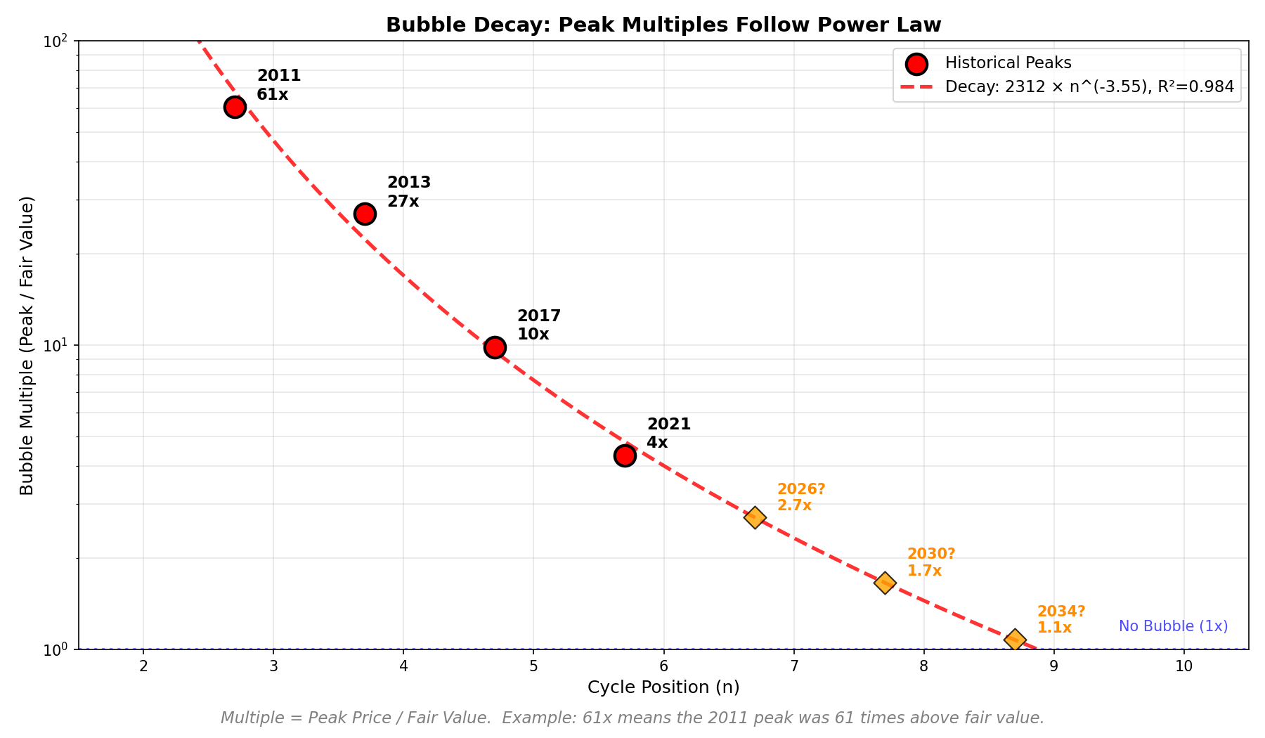Figure 5: Historical bubble peaks (red dots) follow a decaying power law envelope. Each successive bubble is smaller relative to fair value or blue line.

---

Slope Decay: Power Laws All The Way Down

Perhaps the most striking finding: the slope of each bull run (bottom → top in log-price space) follows its own power law decay.

We measure slope as log₁₀(price ratio) per year:

Cycle	Duration	Rise (decades)	Slope (dec/year)	Model
2	295 days	2.66	3.291	3.267
3	742 days	2.76	1.358	1.356
4	1068 days	2.06	0.704	0.727
5	1061 days	1.33	0.459	0.448

The fit is remarkable:

Slope = 0.04 × n^(-2.17)

Three independent power laws now govern the same system:

Component	Formula	Interpretation
Bottoms	price ~ n^b (two-phase)	Floor rises
Peak multiples	multiple ~ n^(-2.87)	Bubbles shrink
Slopes	slope ~ n^(-2.17)	Rises slow down

Power laws all the way down.

This is not coincidence. It’s the signature of a network effect maturing: Metcalfe’s Law (value ~ n²) combined with S-curve adoption dynamics naturally produces nested power laws.

---

Self-Consistent Cycle Projection

Using the extrapolated slope for cycle 6 (0.302 dec/year) we find where the rising price line from the December 2022 bottom ($16,500) intersects the peak envelope.

The constraint: historical peaks occur at approximately 70% of cycle duration.

Iterative algorithm:

1. Guess bottom 7 date
2. Calculate peak envelope at intersection
3. Find where slope line crosses envelope
4. Check if peak is at 70% of cycle
5. Adjust bottom 7, repeat until convergence

Converged result (after 8 iterations):

Parameter	Value
Projected Peak	November 26, 2026
Peak Price	$250,615
Projected Bottom 7	July 30, 2028
Bottom 7 Price	~$84,771
Cycle Duration	5.6 years

Timing Uncertainty

Using ±1σ on the slope extrapolation:

Scenario	Slope (dec/yr)	Top Date	Top Price	Bottom 7
Fast (+1σ)	0.326	Aug 2026	$251k	Mar 2028
Central	0.302	Nov 2026	$251k	Jul 2028
Slow (-1σ)	0.278	Mar 2027	$251k	Jan 2029

Note: price converges to ~$250k regardless of timing. The peak envelope acts as a ceiling; you arrive sooner or later but the roof doesn’t change.

---

Mean Reversion: The Ornstein-Uhlenbeck Framework

Price oscillates between fair value (blue line) and peak envelope (red line). We normalize this as “relative position”:

rel_pos = (log_price - log_fair) / (log_peak - log_fair)

Where:

• rel_pos = 0 → price at fair value
• rel_pos = 1 → price at peak envelope

This transformation creates a stationary series (ADF test p-value: 0.023) that follows an Ornstein-Uhlenbeck mean-reverting process:

dX = θ(μ - X)dt + σdW

Fitted parameters:

• θ (mean reversion speed): 0.00291 (historical average)
• μ (long-term mean): 0.35
• σ (volatility): 0.020
• Half-life: 238 days (~8 months)

The “Yellow Line” at μ = 0.35 represents equilibrium price where the market naturally gravitates absent external shocks. It sits roughly one-third of the way between fair value and peak envelope.

Z-Score Framework

We define Z-score as deviations from the mean:

Z = (rel_pos - μ) / rolling_sigma

Calibrating rolling sigma to produce max historical Z = 4.0 (at the 2021 peak) gives an optimal window of 875 days (~2.4 years).

Current levels (February 2026):

Level	Z-Score	Price
Extreme Sell	+4	~$228k
Target Sell	+2	~$145k
Yellow Line	0	~$92k
Current	-0.85	$62k
Target Buy	-2	~$47k
Panic Buy	-3	~$37k

Interpretation: At Z = -0.85, Bitcoin is slightly undervalued nd below the equilibrium but not at panic levels. The model suggests accumulation is reasonable here, with significant upside to the +2σ sell target.

---

Theta Decay: Bitcoin Is Growing Up

The mean reversion speed (θ) measures how quickly price returns to equilibrium. Analyzing θ over rolling windows reveals a secular decline:

Period	Rolling θ	Half-Life
Historical average	0.00291	238 days
Current (2026)	0.00337	206 days
Projected 2030	0.00292	237 days

Trend: -3.1 × 10⁻⁷ per day

The trend is negative: θ is decaying over time. This means:

• Mean reversion is slowing
• Deviations persist longer
• Volatility is compressing

This is not Bitcoin “dying” it’s Bitcoin becoming boring.

Like gold. Like the S&P 500. Assets that mature don’t oscillate violently around fair value; they grind steadily upward with occasional mild corrections.

The Ornstein-Uhlenbeck Endgame

As θ → 0, the OU equation degenerates to a random walk with drift:

dX = σdW  (no mean reversion term)

This is the standard model for mature assets (Black-Scholes). Bitcoin is transitioning from a mean-reverting speculative asset to a drifting store of value.

Implication for traders: The window for high-volatility cycle trading is closing. Each cycle offers smaller multiples, longer durations, and weaker mean reversion. Accumulate during Z < 0, but don’t expect 10x gains anymore!

---

Synthesis: The Complete Model

Combining all components:

Layer	Model	Purpose
Fair Value	Two-phase power law	Floor (cycle bottoms)
Peak Envelope	Bubble decay power law	Ceiling (cycle tops)
Slope	Power law decay	Rate of rise
Position	Ornstein-Uhlenbeck	Mean reversion within channel
Evolution	Theta decay	Market maturation

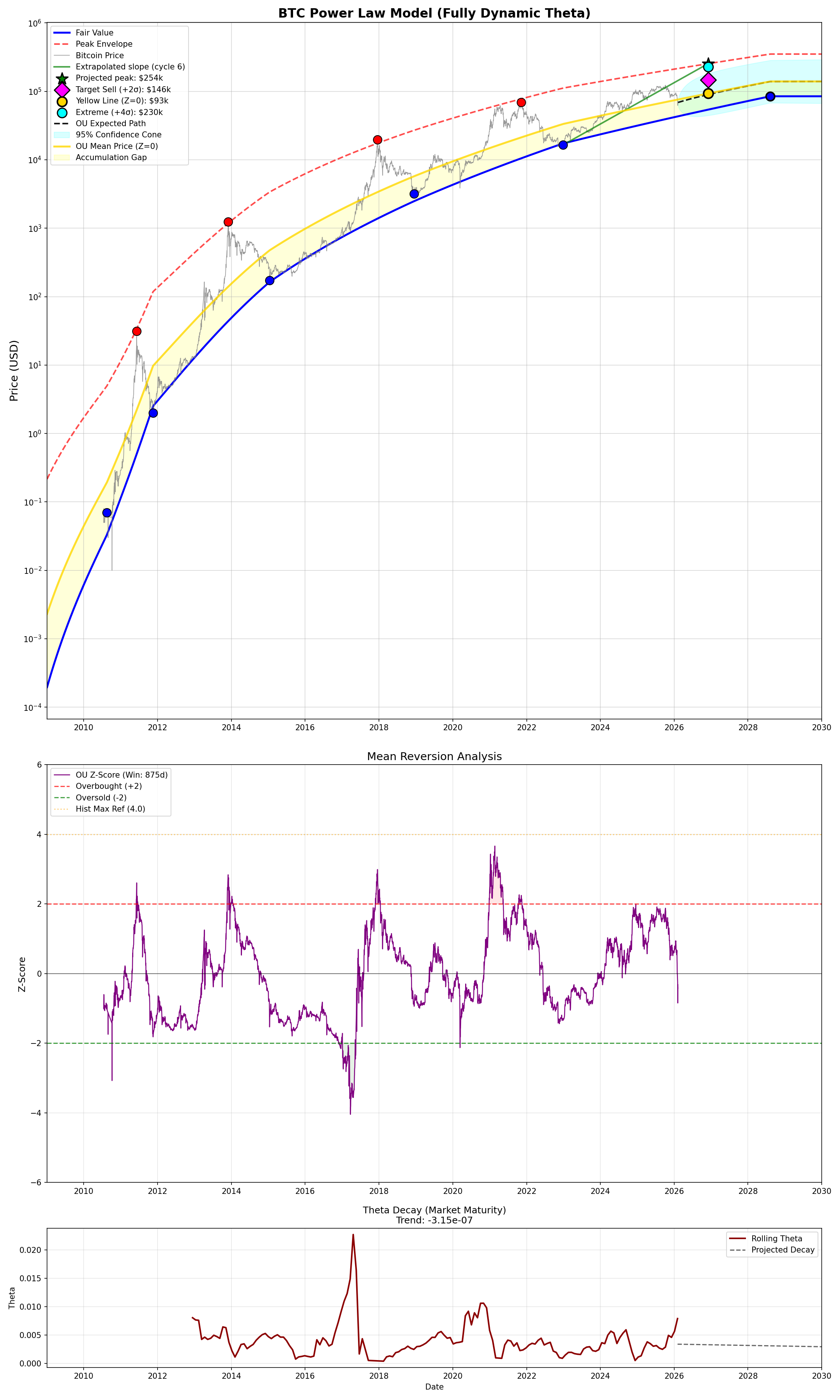Figure 6: The complete model with fair value (blue), peak envelope (red), yellow line (gold), OU projection (black dashed), and 95% confidence cone (cyan). Markers show projected targets at November 2026.

Targets at Projected Peak (November 2026)

Level	Price
Peak Envelope	$250,412
Extreme (+4σ)	$228,083
Target Sell (+2σ)	$145,243
Yellow Line (Z=0)	$92,491
Fair Value	$54,090

Strategy: Scale out between $145k and $228k would be wise. Model shows diminishing returns above +2σ.

---

Conclusions (Part II)

1. Bubble multiples decay as a power law (1078 × n^(-2.87)). Future bubbles will be progressively weaker.

2. Bull run slopes decay as a power law (0.04 × n^(-2.17)). Each cycle rises more slowly than the last.

3. Self-consistent projection points to ~$250k by late 2026, followed by bottom ~$85k in mid-2028.

4. Mean reversion (OU process) provides a framework for Z-score based trading. Current Z = -0.85 suggests mild undervaluation.

5. Theta is decaying, meaning Bitcoin is maturing. Volatility compression will continue. The wild boom/bust era is ending.

6. Power laws all the way down: bottoms, peaks, slopes, and mean reversion speed all follow power law dynamics. This is the signature of network effects maturing.

---

Technical Appendix (Part II)

B.1 Bubble Decay Fit

# Peak multiples
multiples = [60.6, 27.0, 9.8, 4.3]
n_peaks = [2.64, 3.64, 4.75, 5.72]

# Fit: log(mult) = log(a) - c * log(n)
# Result: a = 1078, c = 2.87

B.2 Slope Decay Fit

# Slopes (decades per year)
slopes = [3.291, 1.358, 0.704, 0.459]
cycles = [2, 3, 4, 5]

# Fit: log(slope) = log(a) - c * log(n)
# Result: a = 0.04, c = 2.17

B.3 Ornstein-Uhlenbeck Estimation

# Discrete OU: X(t+1) - X(t) = a + b*X(t) + error
# θ = -b
# μ = a / θ
# σ = std(residuals)

# Results:
# θ = 0.00291
# μ = 0.3501
# σ = 0.02001

B.4 Rolling Theta Trend

# Linear regression on rolling θ values
# Slope: -3.12e-7 per day
# Interpretation: θ decreases by ~0.0001 per year

---

This is not financial advice. Models are tools for thinking, not crystal balls.